Why
The archive has never been seen whole. Regions form here that nobody named — faces along one edge, interiors, dark abstractions, landscape, product. The model was never told what any of these are, who made them, or which project they belong to.
FIELD has kept every reference it collected since 2012. These are the first pictures of all of it at once.
Figures for the “Agency” chapter of New Conditions Vol 01. The archive supports description, not forecasting: it was never published or sampled, so it says what this studio looked at, not what anyone will do next. Failed experiments are hidden; the toggle shows them.
A trend forecast is a claim that things will cluster — that many people will converge on the same thing next season. That is the entire product of an industry.
A private archive can make the opposite claim. It says what one studio actually looked at, unprompted, over fourteen years, with nothing to sell about next season. Nobody outside can reconstruct it, because it was never published. It is the one artefact in the room that makes no forecast at all.
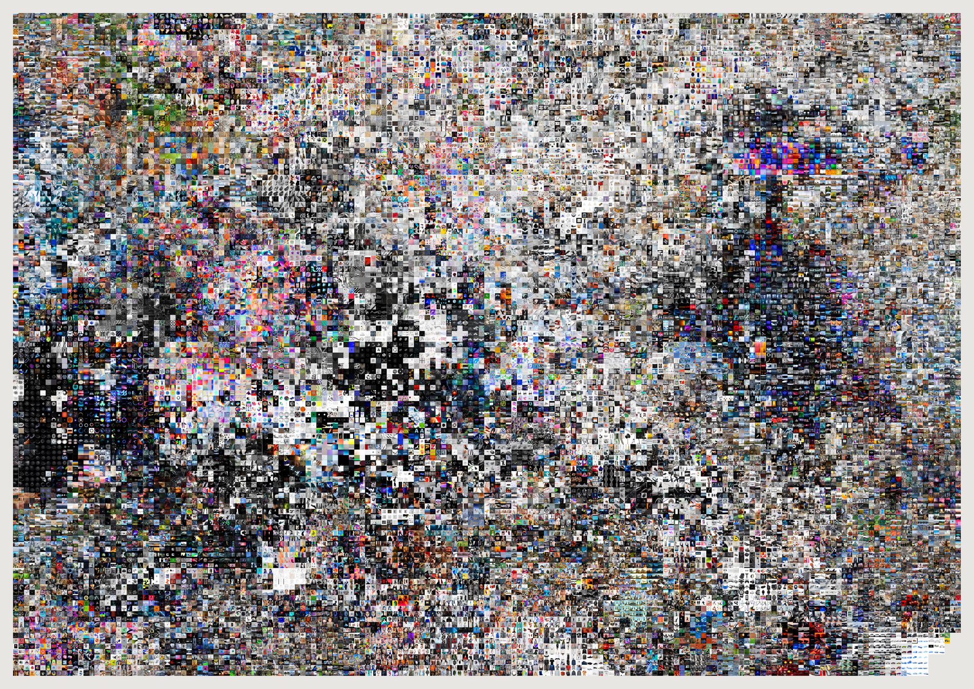
The archive has never been seen whole. Regions form here that nobody named — faces along one edge, interiors, dark abstractions, landscape, product. The model was never told what any of these are, who made them, or which project they belong to.
A raw t-SNE scatter has no reading order, needs a legend, leaves most of the plane empty, and turns its densest regions to mud. Keeping t-SNE's ordering and discarding its coordinates is what makes the form printable.
512-dimension CLIP image vectors, computed locally. Not the text embeddings the archive already had — those were built from scraped captions that often describe the wrong picture.
Two limits, stated rather than hidden. The layout is not stable across runs unless the seed is fixed; t-SNE is stochastic, so a different seed arranges the same relationships differently. And distance across the sheet is not proportional to distance in the embedding — snapping to a lattice deliberately distorts scale to remove gaps. Adjacency is meaningful; measured distance is not.
python3 src/publish.py atlas-everything
# python3 src/viz/atlas.py --max 30000 --page 1189x841 --out atlas-everything
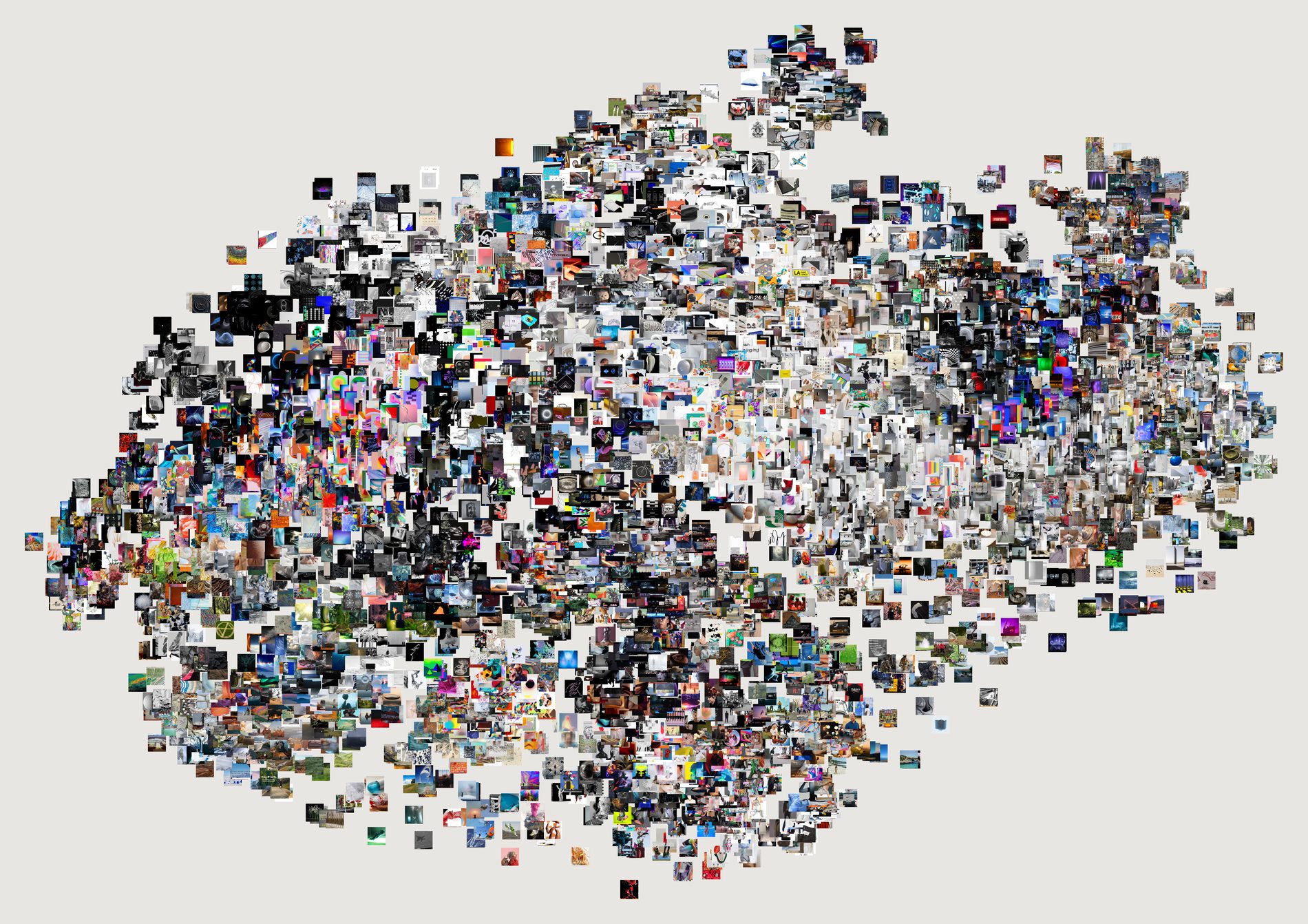
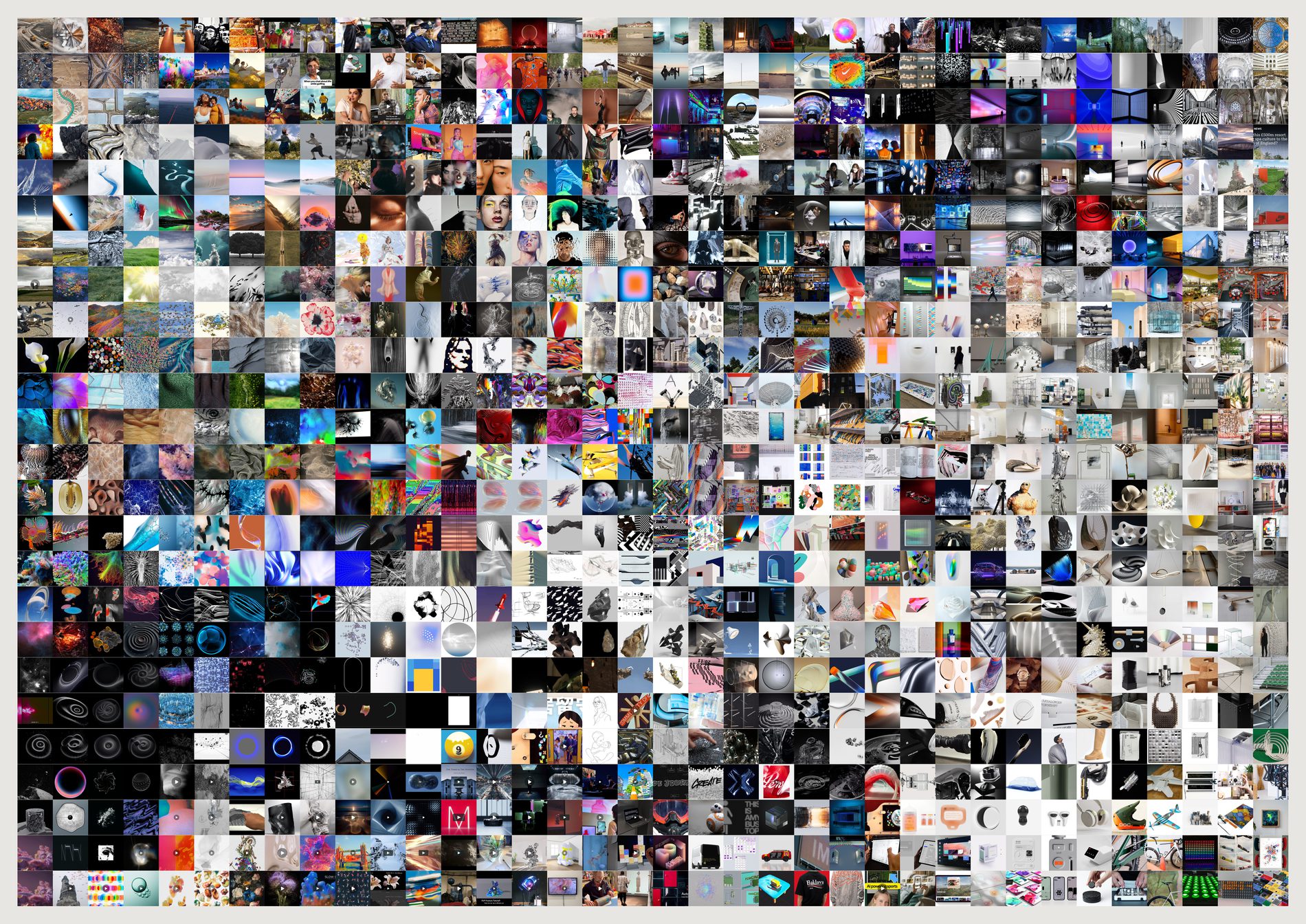
I expected this to be the honest-but-worse version — clusters overlapping into mud, empty plane wasting the sheet. It is worse to read: you cannot reliably find a neighbour, and a third of the paper is empty.
But it is the better image. Organic edge, dense core, a sparse frontier where the isolated references sit. The empty space is not waste; it is the shape of the thing. Gridded is the instrument. Ungridded is the piece. Neither supersedes the other.
Why keep three. The difference between them is the argument for gridding, and it is better seen than asserted. Density is legible in the ungridded one and neighbourhoods are legible in the gridded one; no single sheet does both.
python3 src/publish.py atlas-ungridded atlas
# python3 src/viz/atlas.py --max 6000 --ungridded --page 841x594 --dpi 200 --out atlas-ungridded
# python3 src/viz/atlas.py --max 900 --page 1189x841 --out atlas
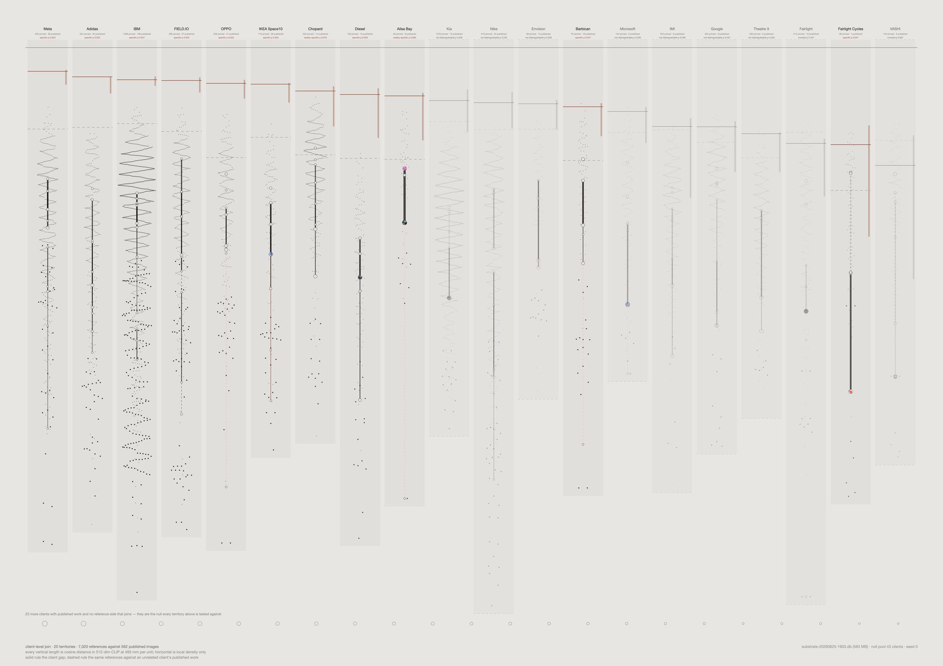
The distance from research to work is smaller than the distance across the research. Reference dispersion runs 0.160–0.274, three to seven times the gap it sits above. And the published cloud is tighter than the reference cloud in 11 of 12 territories, up to 2.94× — the work is a narrowing of the material, not a move away from it.
Vertical length is a real 512-dimension cosine distance at one stated millimetre scale. Horizontal position carries local density and nothing else. Since two t-SNE seeds agree on only 52% of what they draw, this sheet was built so that no claim on it rests on a flattening.
Each client was tested against 43 client output centroids — every client on field.io with three or more embedded published images, including the 27 whose reference side never joins. Four are clear at p ≤ 0.05 where 0.6 would be expected by chance, two more at p ≤ 0.10, and four are indistinguishable from an unrelated client. Nothing survives Bonferroni: the permutation floor is 0.025 and twelve tests want 0.0042. So this is a collective signal, not a per-client licence.
VASHI and Fairlight match other clients’ published work better than their own — lift −0.026 and −0.051, ranking 33rd and 35th of 40. They are drawn as ghosts rather than deleted, because an unevidenced territory is a finding about the join and not an embarrassment to hide.
Opacity comes from each path’s bootstrap standard deviation; a group under three images gets the floor rather than the benefit of the doubt. The 95% interval is drawn as a length, so a 0.184-wide claim looks nine times less firm than a 0.021-wide one. A dashed rule in every territory shows the unrelated-client baseline beside the client’s own.
What this could not do. No project-level relation: channel titles match published work on 2 of 166, so everything here is client-level and labelled as such. And not which way a field moves — direction is only comparable through a shared two-dimensional basis, which is the projection this sheet exists to avoid. Cutting every client to six output images shifts the levels by up to 0.036 but leaves the order at Spearman +0.91, so the ranking survives and the absolute values do not. Only 25 of 66 client pairs have separating bootstrap intervals.
Confidential work is named but never shown. Eight jobs are flagged confidential in the studio's CMS — Mercedes, Apple, Samsung and Google research among them. The client keeps its row here and its references are drawn like any other, because the reference side is the studio's own collecting. What is withheld is the output: 9 published images across four of those jobs are excluded from every sheet in this repo, so nothing FIELD made under an NDA is measured, drawn or published. The count is carried rather than hidden, so a thin published side reads as withheld rather than as absent.
Open the interactive version →
python3 src/viz/translation_field.py --dpi 300

Every other picture here answers a question the designer chose — a facet, a channel, a year, a ranking. The corridor answers a question the viewer chose. Give it two poles and it builds the route on demand, out of the archive, between things nobody at the studio ever put side by side. It is not a generated blend: every cell is a picture FIELD actually pinned.
Open the interactive corridor →
The vectors are unit length, so they sit on the surface of a sphere and the walk follows the great circle. A linear blend cuts through the inside — the midpoint of two vectors 90° apart is only 0.71 long — so after re-normalising the path bunches at the ends and races through the middle. The strip would show movement that was an artefact of the arithmetic.
Once an image is used it leaves the pool. Without that the walk stalls: a dense region is the nearest neighbour to eight consecutive points on the line and the strip returns the same picture eight times. The rule costs something — a corridor through a crowded part of the archive shows more change than the interpolation demands, because it is reaching for the second-nearest.
This was published as a hole, and it is the opposite of one. The number is a cosine between consecutive cells, so a high value means the two pictures are alike and the step is small. The “largest jump” is the run’s minimum cosine — the roughest step on the path — and against thirty random corridors generated by this same script (median worst step 0.741, range 0.570–0.835) all six published walks score higher, mean 0.823, Mann–Whitney one-sided p = 0.00027. These corridors are significantly smoother than random routes through the same archive, and the cell flagged as a hole is the least-smooth point of an unusually smooth path. They are smooth by construction: a walk from subject: person to subject: interior runs between label centroids, the densest regions the archive has, with poles 0.750 apart against roughly 0.59–0.68 for a random pair. What the strip actually demonstrates is continuity — that the archive can be walked from a face to a room in twenty-four steps without a break, more smoothly than chance allows. It cannot locate absence; that needs a route aimed at sparse territory and a null of matched pole separation, and no such sheet exists yet.
A jump is not a hole in the studio's taste — see the correction above. The walk runs over references that are embedded, cached as an image, not a near-duplicate, and not the non-aesthetic material the evidence pool now excludes — 21,491 of 33,455 — so a gap can be an image that was never downloaded. And the strip does not show how far off the line each cell sits: every cell is the nearest available image to a point on the route, and nearest can still be far. The interactive version is one pool behind. It walks a 5,000-reference sample built before the non-aesthetic material was excluded — drawn from 26,214 rather than 21,491 — so it will still hand you the occasional link card, and its jumps run slightly larger again.
python3 src/viz/corridor.py --from-subject person --to-subject interior --steps 24
python3 src/viz/corridor.py --from-mood serene --to-mood dynamic --steps 20
python3 src/viz/corridor.py --random --seed 3 --path
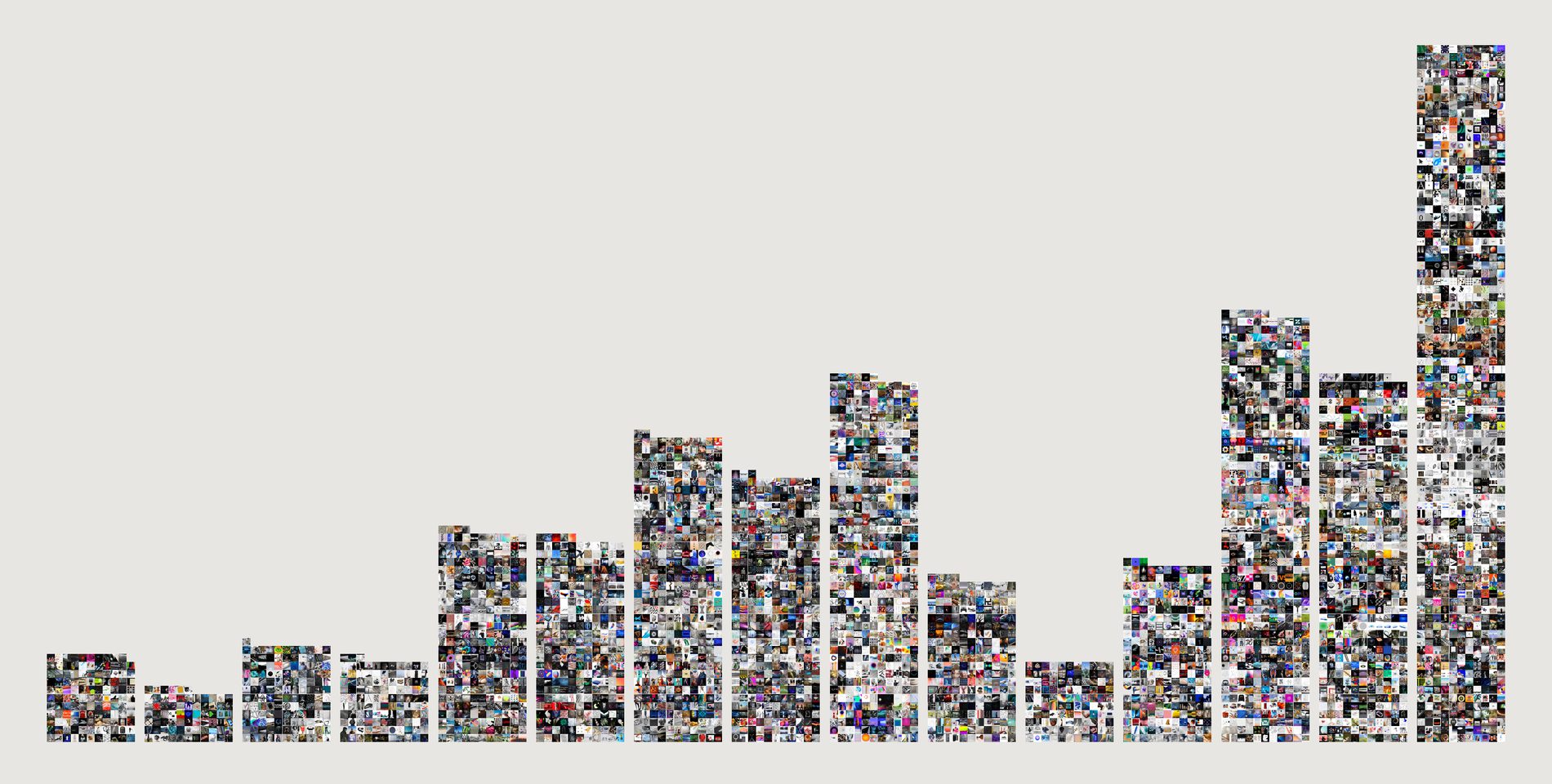
2026 is the tallest column in the archive — 3,675 captures against 2020's 3,168, and it is not a finished year. The studio did not stop collecting.
What collapsed is Pinterest's share: 87% in 2020, 6% in 2026.
In its place: Basecamp 1,461, Instagram 894, manual 412, Figma 144, Notion 45 — and Figma and Notion do not appear as sources at all before 2026.
Pinterest's links went to Vimeo, Behance, Flickr, Colossal, Dezeen. Basecamp's captures are files arriving inside a live project. The move is from browsing to building.
Why this one gets a time axis when nothing else does. The quantity is a count, not a measurement of taste — and a count cannot suffer the thin-tail artefact that killed the other four attempts. The thinness is not a sampling problem; it is the result. What the sheet cannot tell you is whether the studio is looking less, only that it is filing differently.
python3 src/viz/migration.py --page 594x300 --across 11
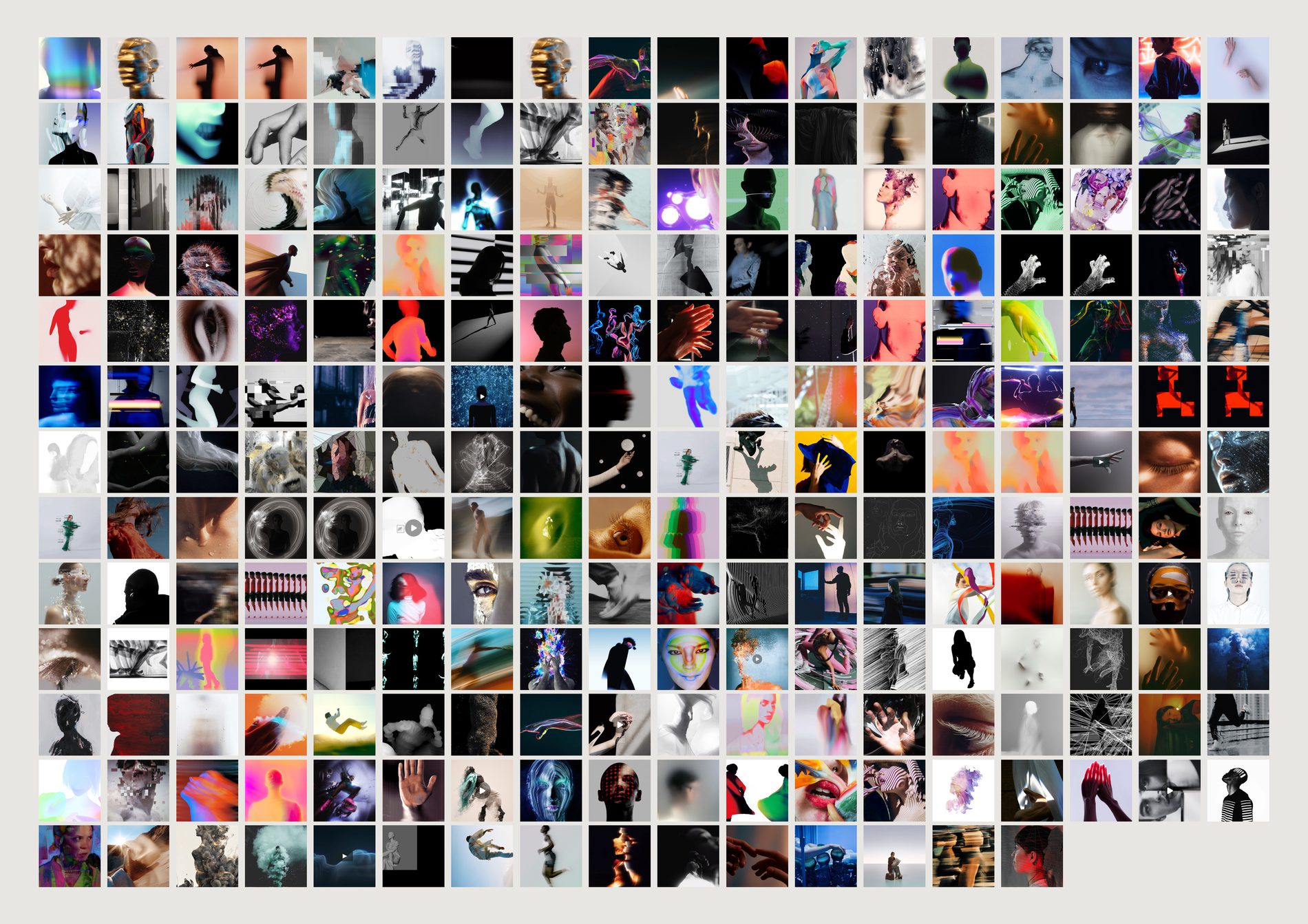
Almost no straight portraiture. Faces dissolved, painted over, distorted, reduced to a single contour.
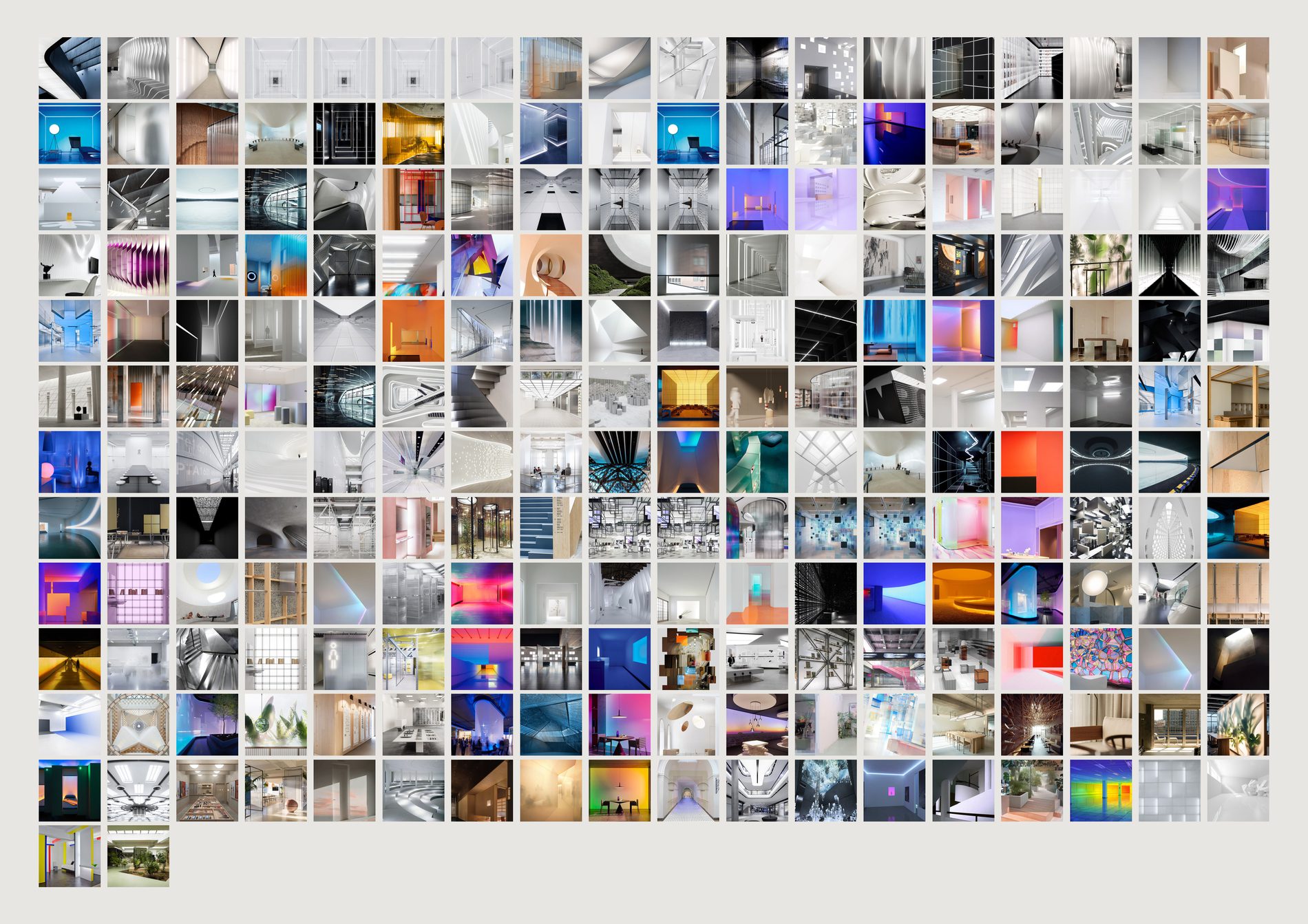
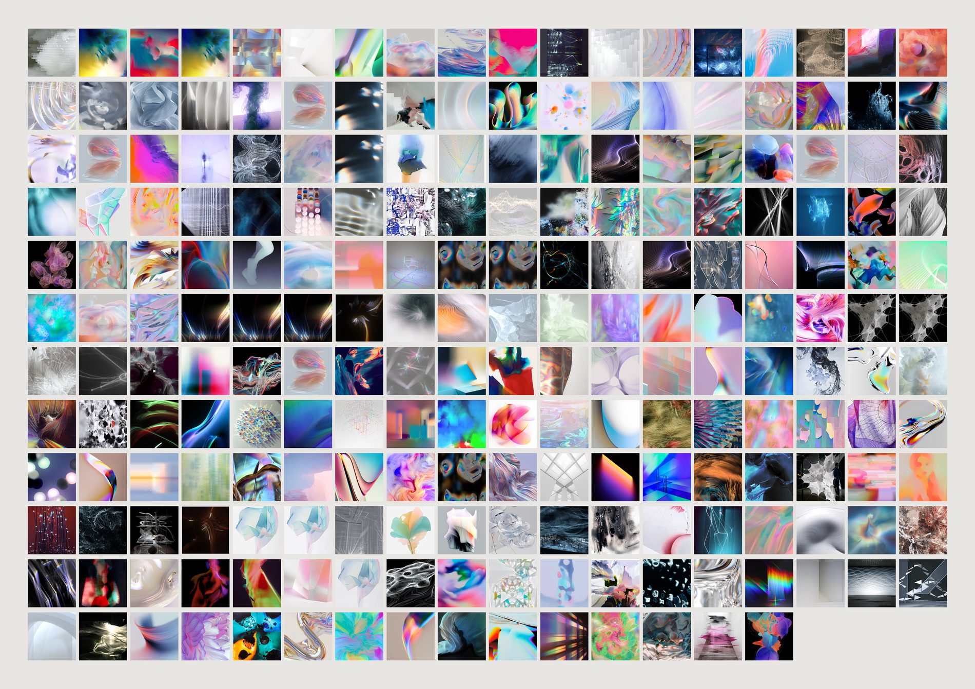
That is a house position on what a person is, and nobody at the studio ever wrote it down.
Images are sorted by distance to the CLIP centre of the category, so the first cell is the most person-like person in the archive and the last only just belongs. You watch a category assemble itself and then dissolve. The edges are the interesting part.
A vision model labelled 30,102 images — 99.9% of everything that has one — with a subject, plus open-text materials, mood and medium. 25 subjects, 879 moods, 690 materials, 24,706 tags. The whole archive was re-labelled on a newer model on 25 August, which is why several counts below have moved since they were first drawn.
The model never saw the channel names. Labelling blind, it reproduced FIELD's own fourteen-year-old taxonomy — see below.
python3 src/viz/facet.py --subject person --sort typical
python3 src/viz/facet.py --mood ethereal
python3 src/viz/facet.py --material glass
python3 src/viz/facet.py --subject person --sort alone   # rarest first
| Channel | Model's dominant subject | Share |
|---|---|---|
| Type | typography | 63% |
| Fashion | fashion | 70% |
| Luminous | installation | 52% |
| Data | data-visualisation | 34% |
| Character | person | 31% |
| Form | sculpture | 27% |
| Space | interior | 23% |
Counted over every labelled reference in each channel, not over the taste pool — the question is what the folder holds, not what counts as evidence about the eye. These seven shares are unchanged by the pool rewrite. One row is weaker than it looks: Data's dominant subject is data-visualisation at 34% over the whole channel, but inside the pool it drops to 21% and ties with abstract, because much of that board is charts with words on them.
This does not make every individual label correct. It does mean the categories were describing something real rather than being arbitrary buckets — which is worth knowing before anyone builds on them.
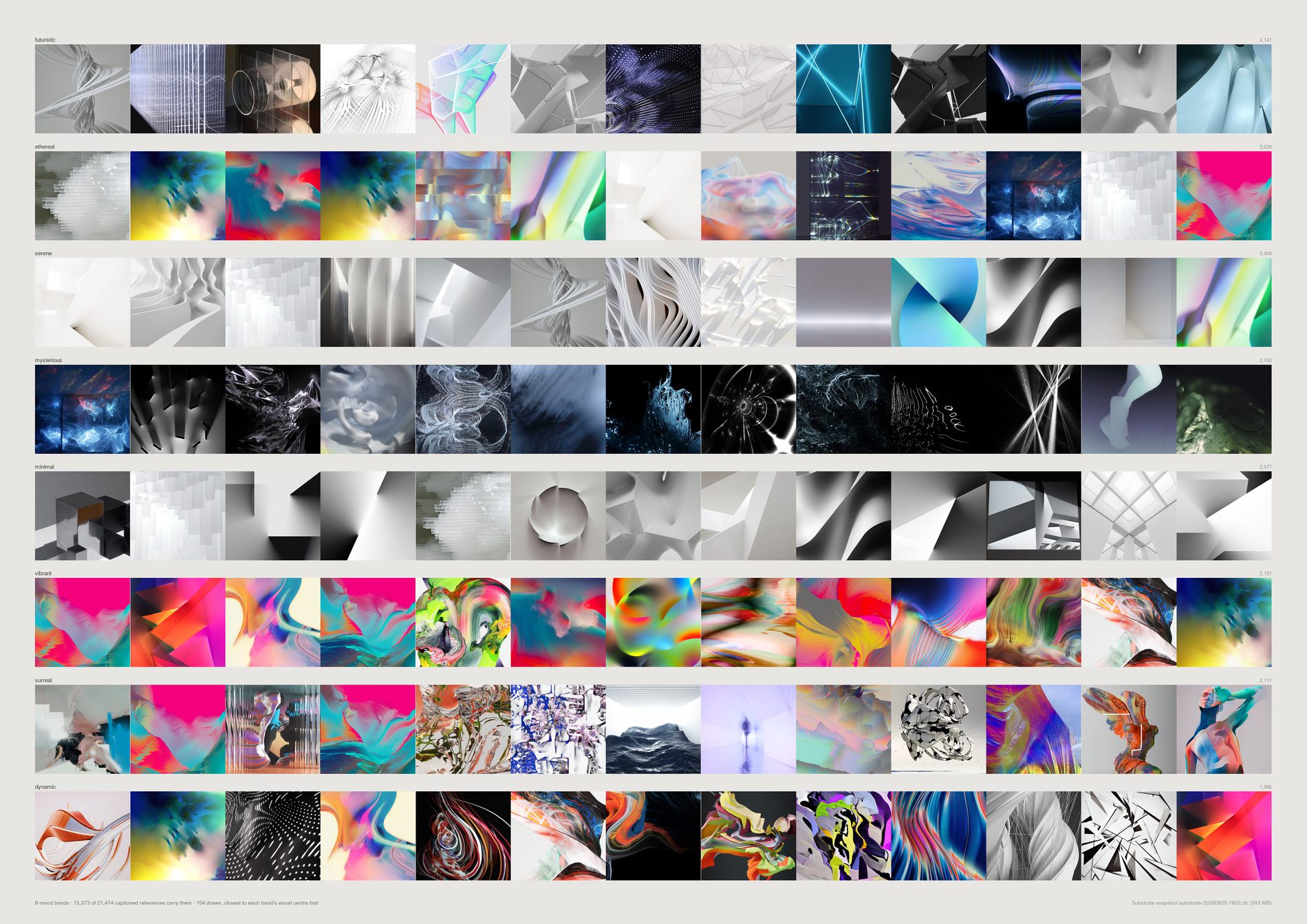
ethereal 2,968 · serene 2,169 · mysterious 2,094 · vibrant 1,940 · dynamic 1,915 · calm 1,622 · playful 1,552 · minimal 1,467
Luminous reads ethereal and mysterious. Character reads mysterious and surreal. Space reads serene. Fashion reads edgy. Data reads analytical. Each channel has a mood signature nobody assigned it.
metal 4,427 · plastic 4,323 · glass 3,240 · fabric 1,608 · paper 1,273 · wood 1,133 · concrete 1,088 · light 982 · paint 833
FIELD barely looks at nature. sky 0.7% · water 0.6% · landscape 4.9%. Installation, abstract, object and sculpture together are 44%. Made things, in rooms. And 65% photographs against 27% renders — the real over the simulated, better than two to one. Measured over the 16,326 labelled references in the evidence pool.

Over all 43 registers with 60+ pooled references: IBM Think 2020 0.819 · FIELD-Next Identity 0.817 · Parametricism + Materials 0.816 · Dolby 0.808 · PG2 0.806. The identity and installation work is where FIELD looks most like itself.
Diesel Digital Nature SS16 0.684 · P332 NikeTown London 2027 0.691 · P062 Dystopia987 0.701 · FIELD x Fairlight Cycles 0.717 · FIELD-X: Aerosolar 0.726.
Widest, by lowest internal coherence: P332 NikeTown 0.721, Dystopia987 0.723, Diesel Digital Nature 0.726, Aerosolar 0.742. Narrowest: Parametricism + Materials 0.842, Barbican Virtual Realms 0.834, FIELD-Next Identity 0.831. The pitch and exploration boards are where the range is; the material and identity boards are the tightest.
An inversion worth investigating. DeepTime is the tightest board in the bottom half — internal coherence 0.829, but only 0.741 to the house. It is the largest gap on the sheet between how consistent a board is with itself and how much it resembles FIELD's own eye, and it is self-initiated, so nobody's brand pulled it there. A question rather than a law.
The sheet draws five registers; the rankings above are over all 43. Re-run with --n-clients 43 to see the whole table. The earlier version of this section quoted a split-half ρ of 0.77 that nothing in the repo computes; it has been removed rather than carried forward unverified.
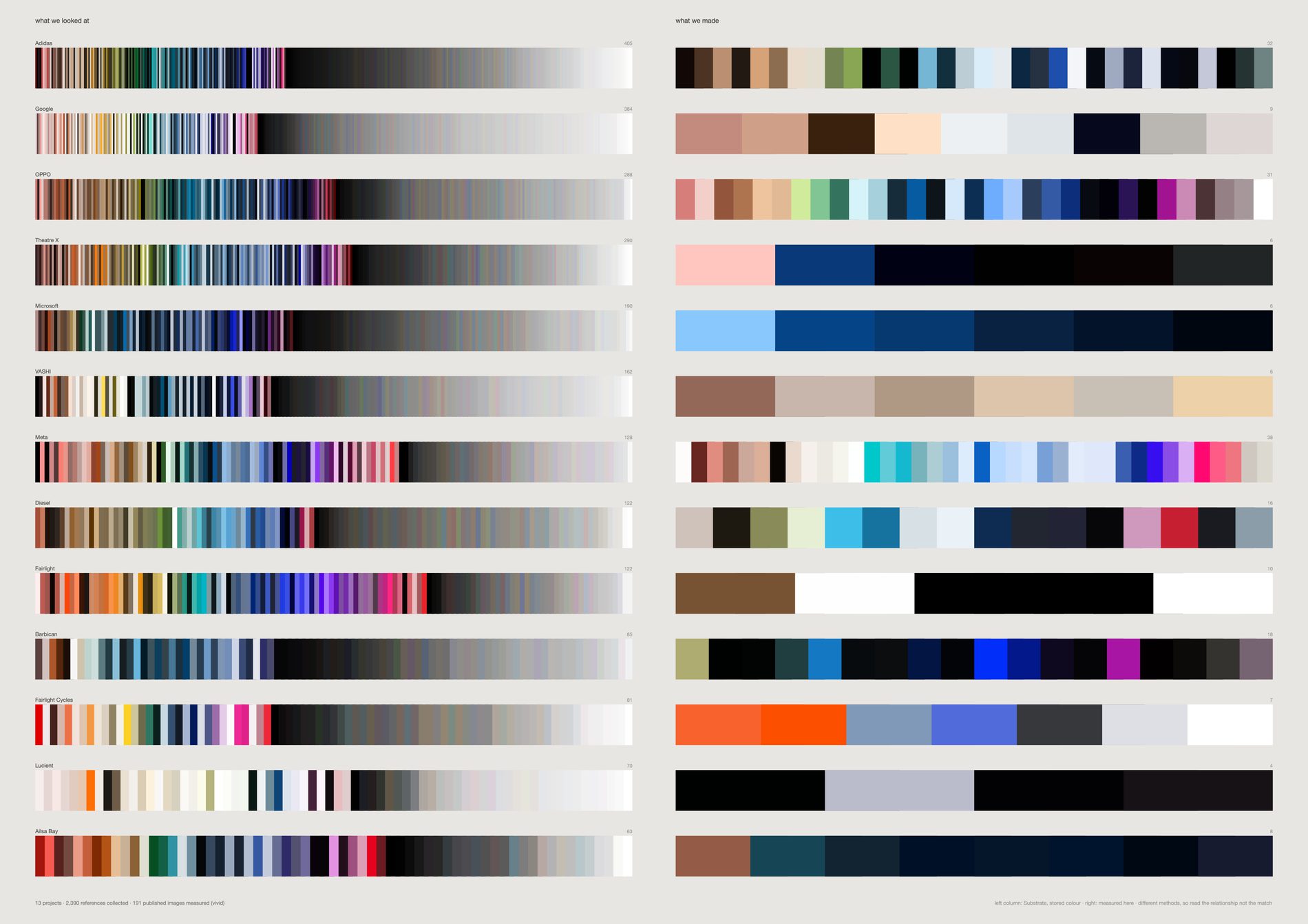
The right-hand column is public — it is on the website, it has been indexed, any model trained on the web already holds it. The left-hand column exists nowhere outside this studio and is not recoverable by running the finished work backwards. The asymmetry is the content.
The two sides are not measured the same way. The left uses colour computed upstream years ago by a method that tracks the image mean; the right was measured here, taking the most saturated significant cluster. The sheet is about relationship, not equivalence.
The gap, three ways. A pass over that sheet asked whether it is superseded by the translation field or by lineage, and concluded it is not: both successors normalise volume away, and nothing else in this repo says how much more looking there is than showing. The same pass found two defects in the sheet above, neither of them fixable inside it. Both columns are drawn the same width, so Lucient's 4 published images occupy exactly as much page as Adidas's 347 references — confidence is drawn inversely to evidence, and the count that carries the whole asymmetry is printed at 2.2pt. And hue-sorting collapses any set past about two hundred colours onto the same ramp, so thirteen studios' worth of research reads as thirteen near-identical ribbons, which is a property of sorting rather than of the archive. The three sheets below give up the like-for-like colour comparison — which the caption above already disowns — and draw the ratio, the reach, and the material instead.
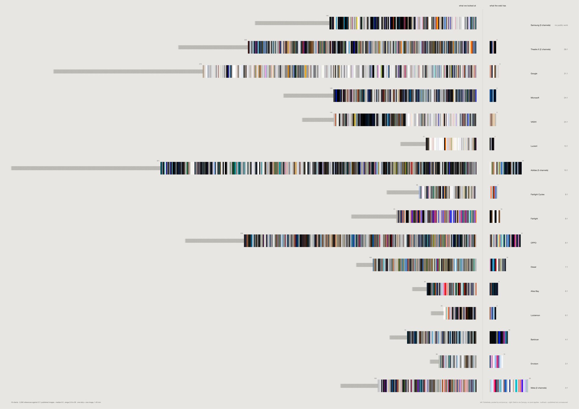
Across sixteen client relationships the studio holds a median of 8.4 reference images for every image it published, running from 2.7 at Meta to 39.8 at Theatre X.
Google is 307 against 9, Adidas 347 against 32, VASHI 146 against 6. Samsung is the limit case and it is drawn: 161 references, nothing public at all, so its right side is empty.
There is no projection, no normalisation and no axis anywhere on this sheet. The scale is the same on both sides of the rule and the same on every row, so a band's length is its count — which is the one comparison the equal-width version made impossible.
Within a band, references run in the order of the material's own date. So a band reads as the history of one relationship rather than as a spectrum, and the thirteen identical ramps problem disappears with the sorting that caused it.
Beyond each solid band on the left sits what src/pool.py removed — 680 near-duplicates and non-aesthetic references across the sheet. Drawn rather than deleted, because what a filter costs should be visible on the sheet that benefits from it.
A published image that exists but whose colour could not be measured is drawn as an empty outline rather than dropped — here that is one image, on Meta. Archive-wide, 437 of 1,464 published images 404 or time out on Cloudinary, and outlining them stops the right column from silently shrinking to whatever happened to download.
What would make this wrong. The right column is what was shown, not what was made: field.io publishes a selection of images from a selection of jobs, chosen for taste and for client approval, and the true denominator is in no database here. So the ratio is an upper bound on what is public and says nothing about the studio's own delivery archives — the objection that does the most damage, and it cannot be answered from these two sources.
The left column is not the whole record of looking either. It is the references filed into a channel that names the client, surviving the pool, carrying a stored colour; work done for a client without a Substrate channel does not appear, and 87% of the archive came off Pinterest, whose ranker shaped most of what was available to choose from. The join is by client name, not by project — titles match on 2 of 166 channels, so Adidas folds five channels and Meta two, and a row is about a relationship rather than a brief. And a ratio is not a rate: nothing here says the studio needs nine references to make one image. Both sides accumulated over fourteen years by different processes, and the reference side kept growing after the work shipped.
python3 src/viz/gap_scale.py --page 841x594 --dpi 300 --out gap-scale-a1
# python3 src/viz/gap_scale.py --list   # the counts, recomputed on every run
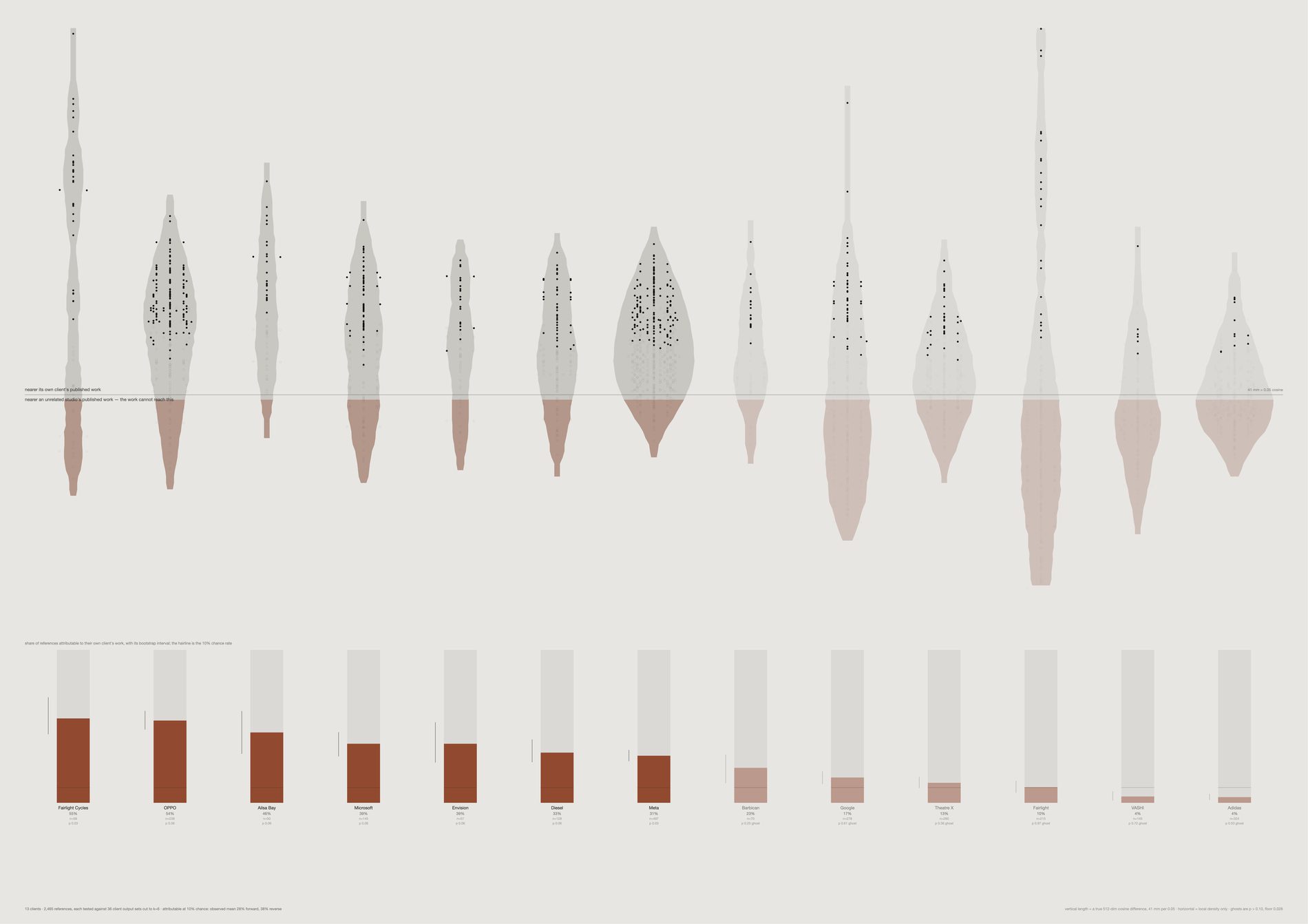
The sheet above asserts that the research is not reconstructable from the outputs, and nothing in this repo measured it. Here every dot's height is a difference of two true cosine distances in 512 dimensions: its distance to the nearest of six images published by a stranger, minus its distance to the nearest of six published by its own client.
The reverse direction is computed at the same k against the same style of null — the share of published images attributable to their own client's references — and it comes out at the same level. Forward 29%, reverse 29%. The link runs both ways at about three times chance and accounts for under a third of the material in either direction. The asymmetry this archive carries is one of volume, not of reach, which is what the scale sheet draws. Claiming a directional asymmetry would be drawing something the data does not hold, so the caption on the sheet says so.
The horizon at zero is exactly “as close to an unrelated studio's published work as to the work it was collected for”.
29% of collected references are attributable to their own client's published work, against a chance rate of exactly 10%. Roughly three times chance, and it leaves the great majority of the research invisible from the public side — measured rather than asserted.
Nearest-neighbour distance falls as a set grows, so a client with 39 published images would beat one with 6 for a reason that has nothing to do with the studio. Every output set here, the client's own and every null, is cut to the same k and averaged over resampled draws. Anything comparing two different kinds of quantity on this sheet is a bug, not a finding.
Only 2 of 13 clients clear p ≤ 0.05 — Fairlight Cycles and Microsoft, both at p 0.03. Seven do not clear p ≤ 0.10 and are drawn pale with the word ghost against them. Nothing indistinguishable from an unrelated studio is drawn as though it were a finding.
Width inside a territory is local density and nothing else — a territory is wide where many references sit at that depth. Every vertical length is a real cosine difference at the millimetre scale printed in the caption. There is no projection on this sheet.
What would make this wrong. Nothing here survives a Bonferroni correction. With one test per client the family wants a p far below what a permutation over this many strangers can produce — the floor is 0.032 — so a handful of hits where one is expected by chance is a collective signal and not a per-client verdict.
The attributable fraction tracks reference count, in the uncomfortable direction: Spearman −0.40, the biggest collections scoring lowest. A large, wide-ranging board is more diffuse, so less of it lands near any six images, and some of the spread on this sheet is that rather than the studio. The second digit is not stable — the attributable share is an average over resampled draws, and re-running --list returns a mean of 25% against the sheet's 29%. Read the ordering, not the decimal. The published side is a curated subset, so an unattributable reference may have fed something that was made and never shown. And CLIP is one instrument: the stability sheet found orders survive a change of encoder at rank correlation +0.95 while levels shift wholesale, so the ranking of these territories is the result and the absolute fractions are a property of this model.
python3 src/viz/gap_recovery.py --page 841x594 --dpi 300 --out gap-recovery-a1
# python3 src/viz/gap_recovery.py --list   # every client's fraction, interval and p
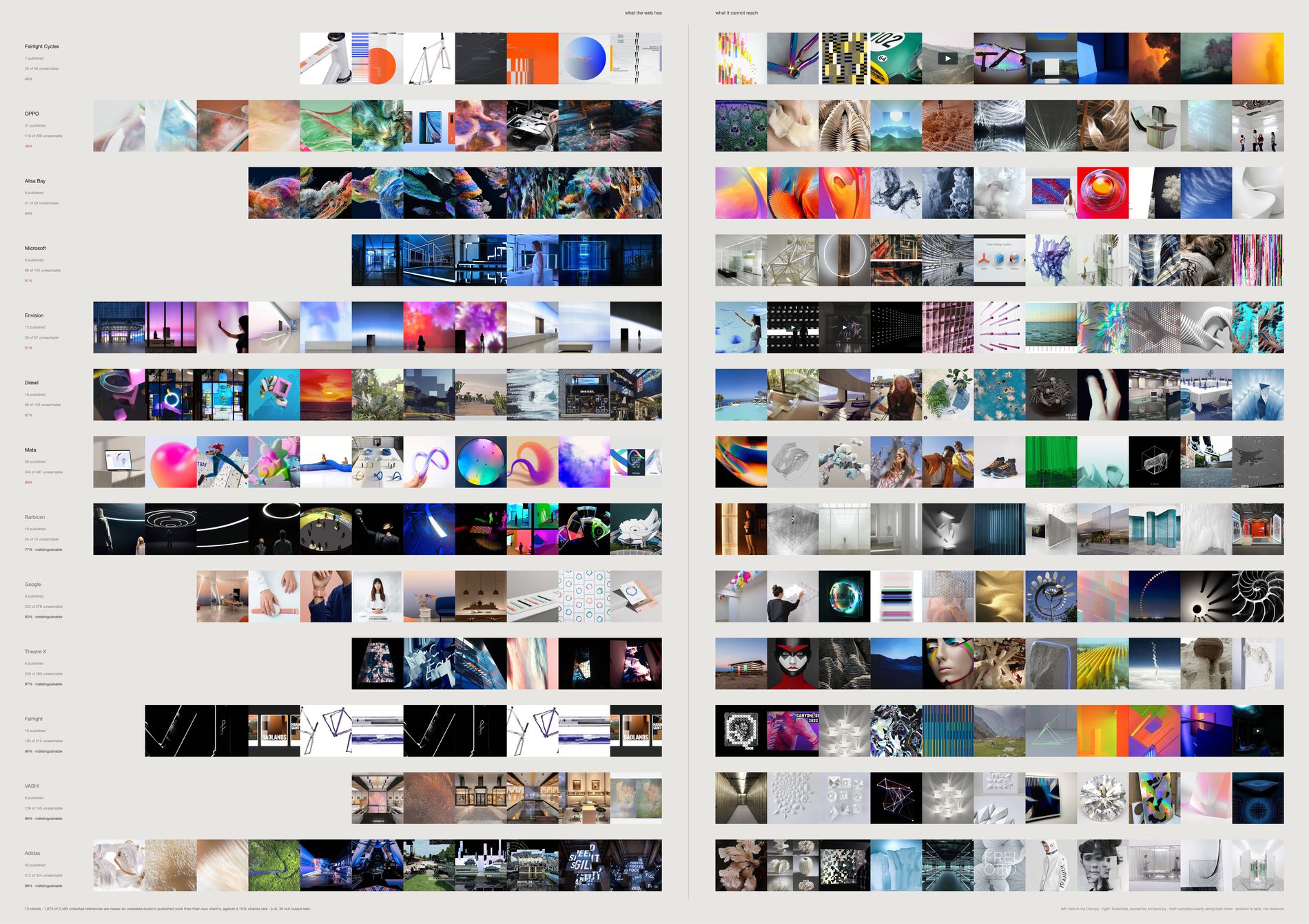
Left of the rule: images FIELD published on field.io — public, indexed, already inside any model trained on the web. Right of the rule: references collected for that same client which are measurably nearer an unrelated studio's published work than their own client's.
The selection on the right is a measurement, not an edit.
Per client it runs from 39% at OPPO to 97% at Fairlight. Adidas is 334 of 350, Google 240 of 307, VASHI 139 of 146. Put the two halves side by side at the same size, with the right-hand side chosen by a test rather than by an editor, and the two columns do not look like each other — which is the one form of this argument a reader can check by looking.
The images shown are drawn evenly along the whole unattributable order, from the references that only just failed the test to the ones furthest from anything the studio published. The typical sheet established for this repo that the single item at the end of a ranking is a design decision dressed as a measurement, so nothing here is the extreme case.
Horizontal position is rank in the measured order. There is no projection on this sheet and no distance on it can be read with a ruler.
Adidas reads 95% unreachable here and 0% unmatched on its own territory, and both are correct. That sheet counts a reference as unmatched when its centroid similarity puts it nearer at least half of thirty-nine other clients' published work; this one when it beats fewer than 90% of thirty-one strangers on nearest-of-k distance. A median threshold and a 90th-percentile threshold on two different statistics are not the same test.
What would make this wrong. A sample is not the set — eleven images stand in for thirty to three hundred, and though the sample is even along the ranking it is still a sample; raise --per-side or change --seed before quoting any row. Unattributable is not unrelated: photographs of interiors sit near other photographs of interiors, so a reference can fail this test and still be the reason a job looks the way it does. What the sheet shows is what the published work cannot account for, which is weaker and more defensible than what it did not cause.
Seven of thirteen clients do not clear their own permutation test and carry the word indistinguishable beside their percentage; on those rows the split between reachable and unreachable is not distinguishable from what an unrelated studio would produce. And the play buttons on some right-hand cells are a known hole: aesthetic.py filters on media type and the vision model's made label, so an Instagram or Vimeo still with interface burnt into it is neither a link nor labelled typography and passes through, then sits far from photographs for a reason that has nothing to do with taste. Putting the pictures in is what makes that hole visible; the colour and dot versions of this sheet hide it.
python3 src/viz/gap_unreachable.py --page 841x594 --per-side 11 --dpi 300 --out gap-unreachable-a1
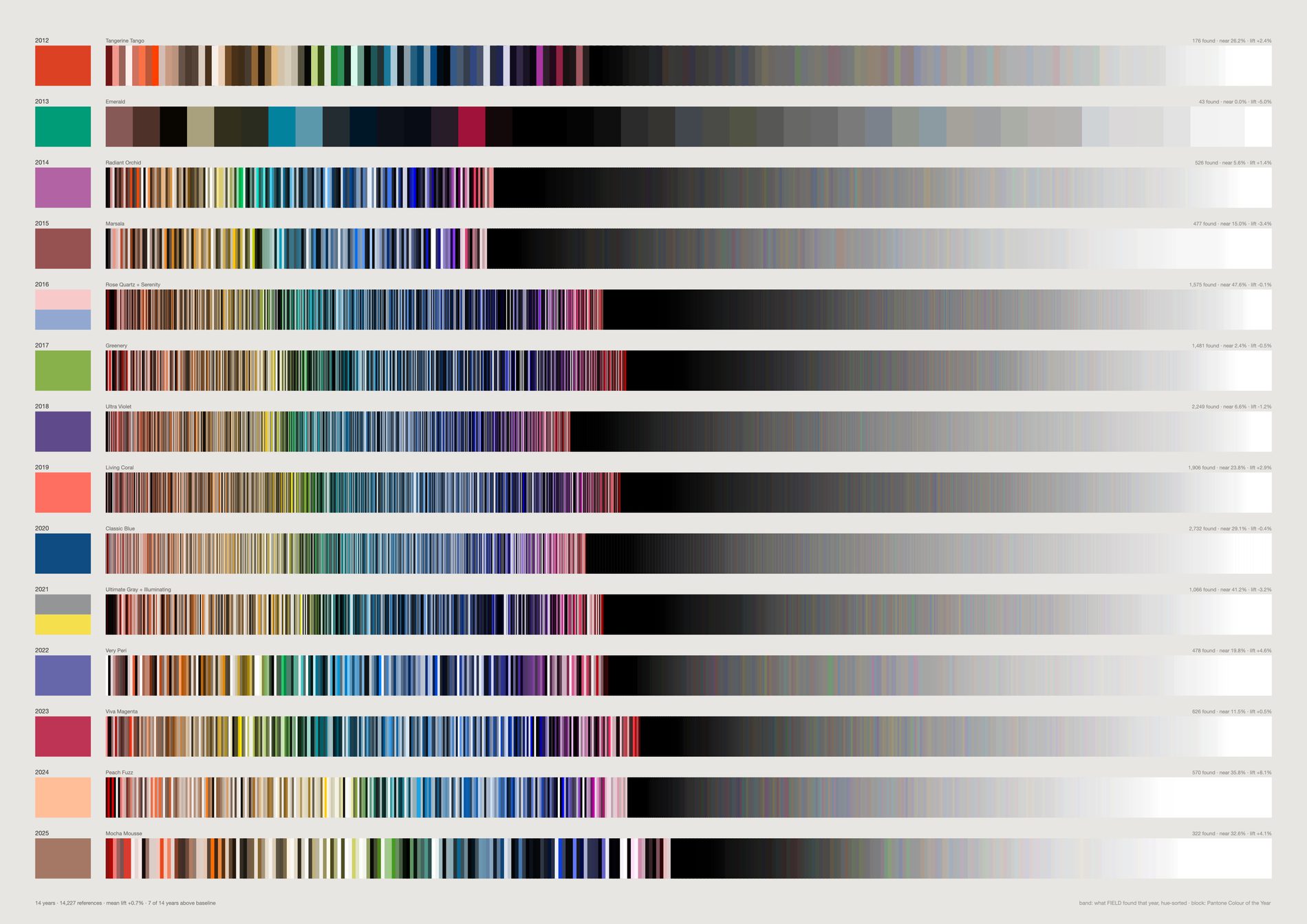
Seven of fourteen years above baseline is a coin flip. FIELD's palette shows no relationship to Pantone's annual forecast. In the year of Greenery the archive went slightly less green; in the year of Classic Blue, slightly less blue.
The industry has already conceded the mechanism. Pantone's own press release says the Colour of the Year “has influenced product development and purchasing decisions” — a claim to have moved the market, not to have foreseen it. Heuritech advertises +91% accuracy at 24 months; its own peer-reviewed paper reports 51.0% three-class accuracy at 12 months against a 35.7% baseline.
2026 is deliberately absent. Pantone has announced it; it could not be verified from a source here, and nothing on these sheets is drawn from an unverified value.
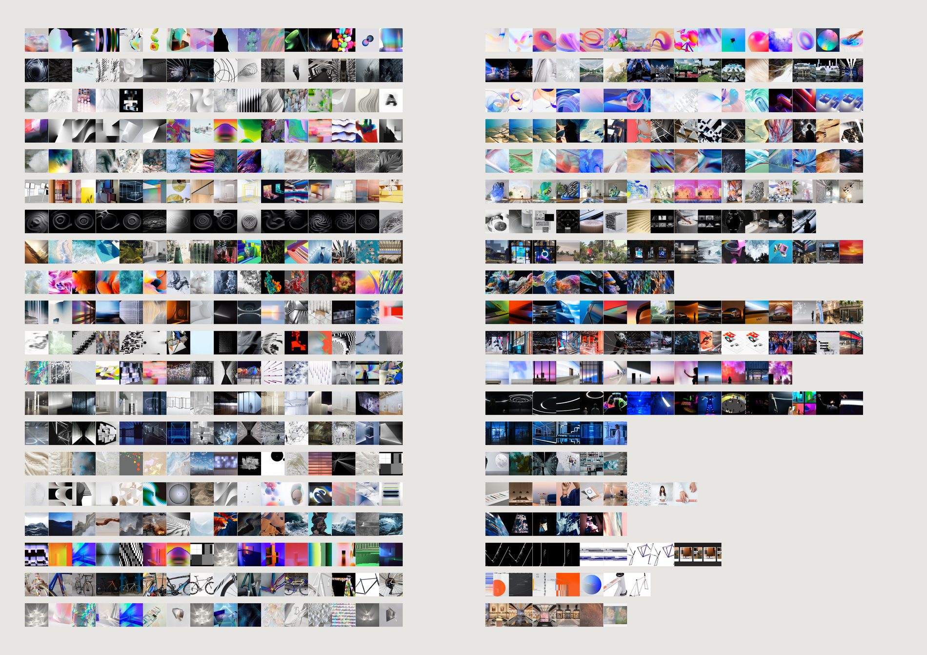
The colour version had to caption itself with a warning: the two sides were measured by different methods years apart, so it could only show a relationship, never a match. Both halves are now CLIP image embeddings from the same run.
The cosine between the two centroids. High means the work came out looking like the research. Low means something happened in between that the references do not explain — and that gap is the studio's own contribution.
Adidas 0.962 and OPPO 0.955 at the top; Fairlight 0.818 and VASHI 0.849 at the bottom. Fairlight's row is the one to look at: vivid colour-field interiors on the left, black-and-white line work on the right.
Two things that would make this wrong. The join is by client, not by project — titles match on 2 of 166 channels, so a client with several jobs has both sides pooled and the row is about a relationship rather than a brief. And published images are already filtered by taste and client approval, so the right column is what was shown, never what was made.
python3 src/viz/lineage.py --page a2l --per-side 16
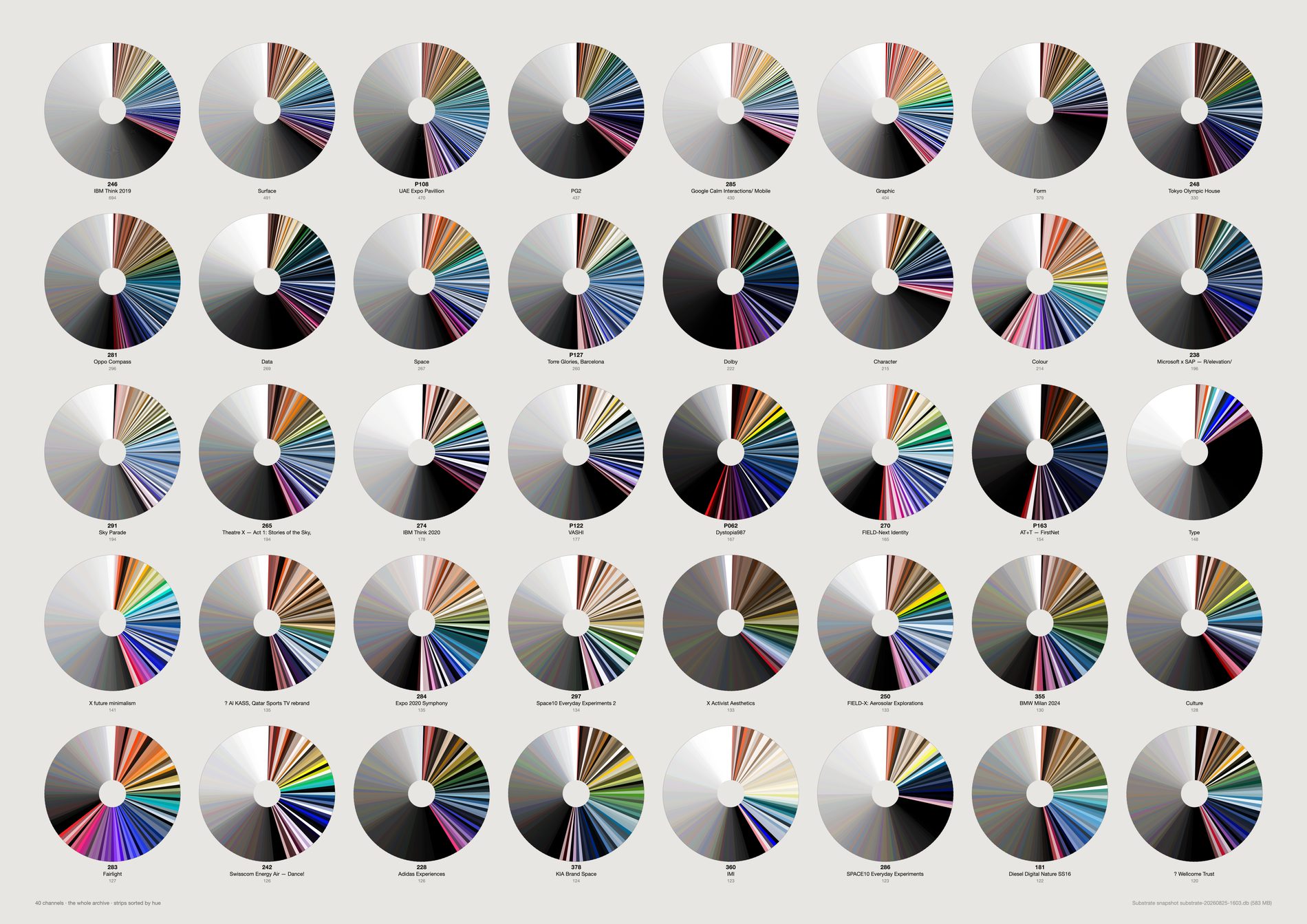
The palettes match the briefs. Google Calm Interactions is the palest channel in the archive (67% neutral); Dolby the darkest; Fairlight the most chromatic; Type is 84% neutral.
The archive encodes what each job was about.
Form warning. This is close to Jason Salavon's territory — his Field Guide to Style & Color (2007) reduced the entire IKEA catalogue to colour and structure as a 374-page book. If this form is used, the ordering has to be the finding rather than the decoration.
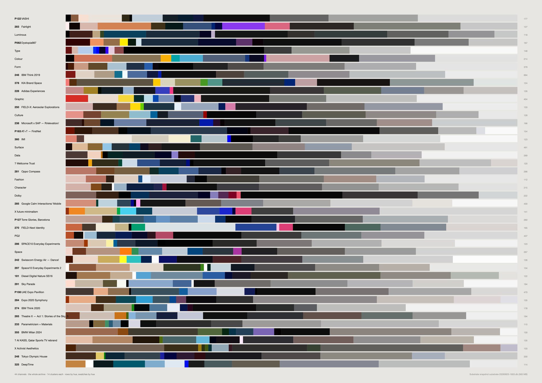
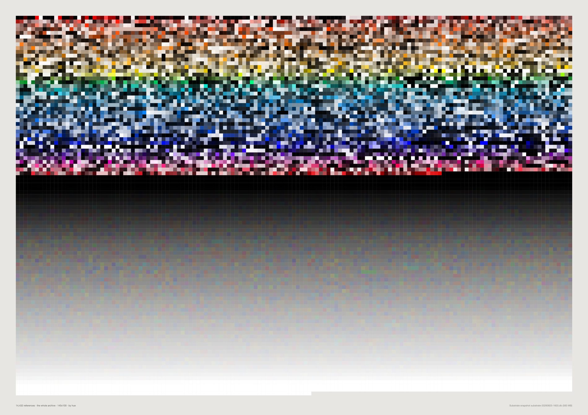
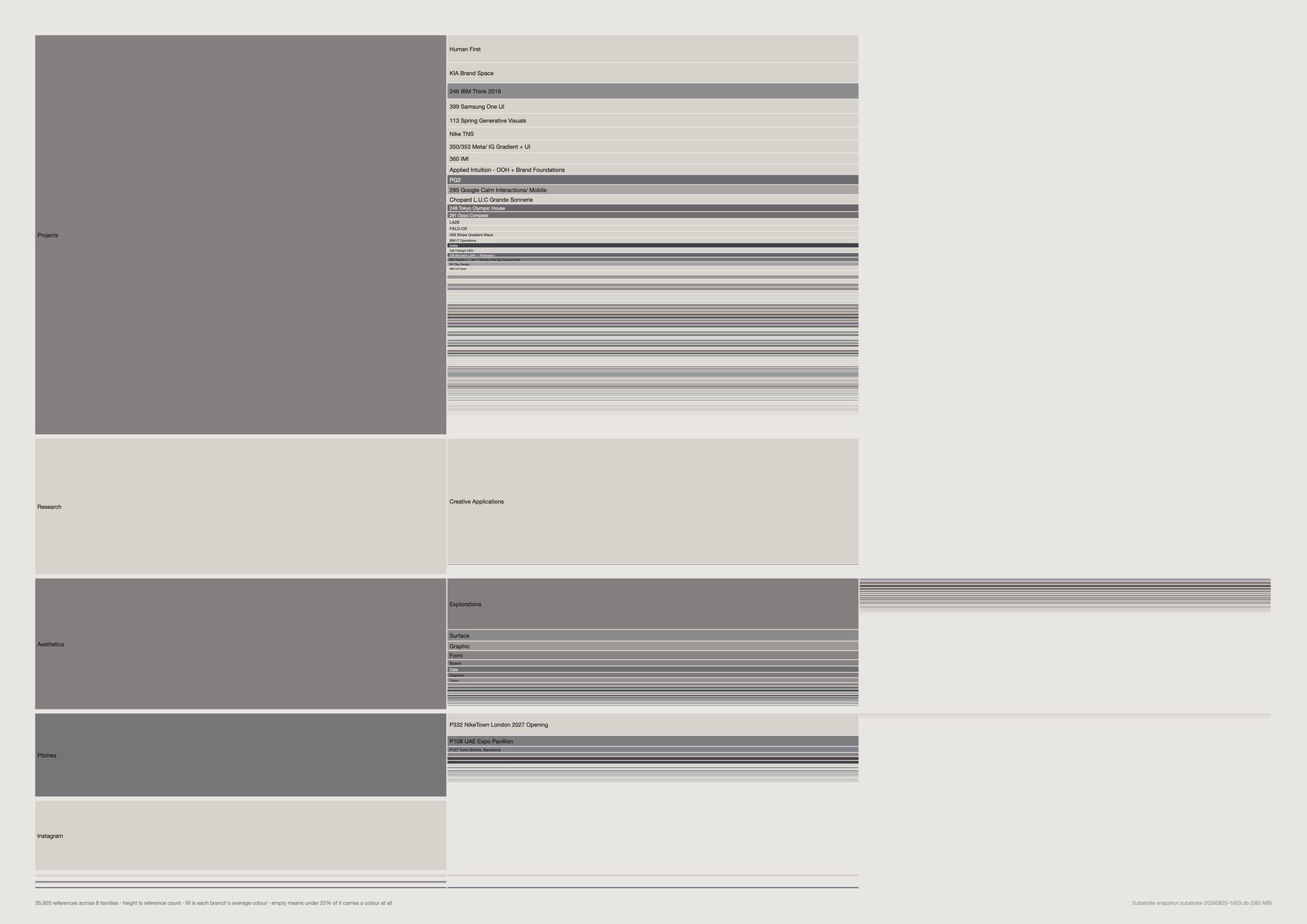
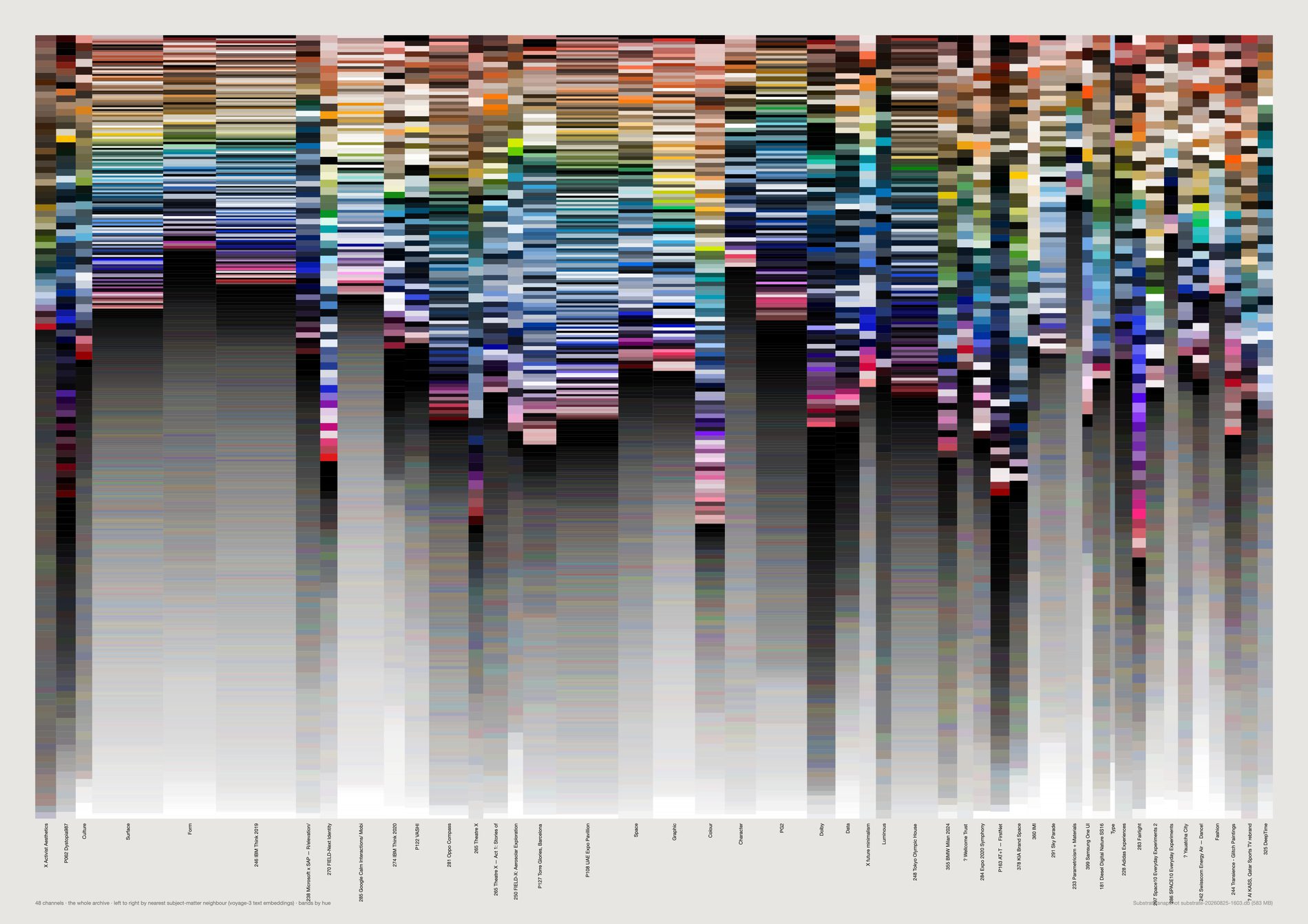
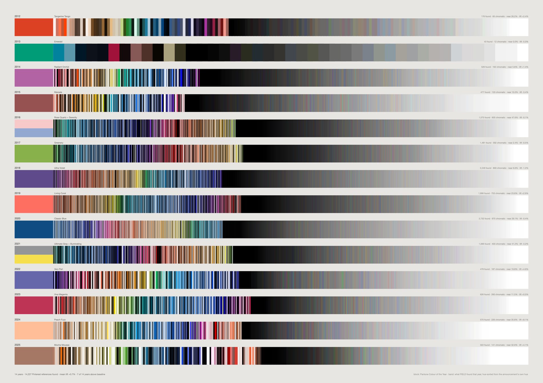
This differs from the test above in two ways that make it the argument rather than the analysis: no gutter, so block and field meet at a hard edge; and the field is anchored at the Colour of the Year's own hue, so the announcement gets the best seat in every row. What sits there is a few millimetres before the year goes elsewhere.

A taste has a centre and a frontier. The page is 1200×48mm because a single row of n cells is n times wider than it is tall — on A2 it renders as a hairline in an acre of paper.
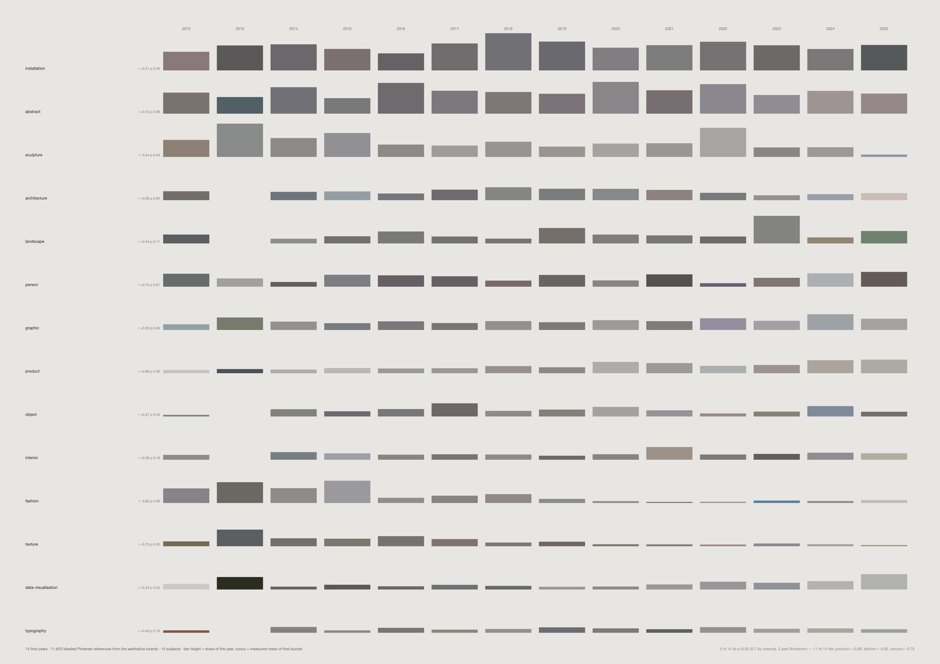
Twelve of fourteen subjects are flat, as expected. Fashion is not, and neither is texture.
Fashion runs from 11.1% of the studio's early finds down to 0.6%, at r = −0.85; texture from 11.1% to 2.1% at r = −0.79. Those are the only two that survive a Bonferroni correction across fourteen tests.
And the mechanism deflates the headline one. The Fashion board's last real year is 2019, while Surface, Graphic and Colour are still being pinned in 2025. The studio stopped keeping a fashion board. That is a change in what it looked at and worth saying — but it is board lifecycle, not the eye evolving.
The vision pass has since been run over four times as many images as when this was first drawn — 10,816 labelled Pinterest references against 4,022 — and the shape held.







The largest jump is where the nearest available image is furthest away — the point at which the line passes through territory nothing in the archive occupies. It is a measured hole in fourteen years of looking, and the piece finds it without being asked.
Chosen poles jump between 0.809 and 0.843. The random pair jumps at 0.781 — still the roughest walk on the sheet, but only just. That gap has closed since the sheet was first drawn, and the reason is the archive rather than the method. Over 21,491 references a random pair jumped at 0.571 against 0.808 for chosen poles, and the claim read as obvious. Over 21,491 the arbitrary line finds a near neighbour almost as easily as a considered one, because the recovered Figma material filled in the ground the old corridors had to leap. The direction survives and the size of it does not.
Slerp, not linear interpolation — these are unit vectors, and a straight line through the sphere cuts the chord rather than the arc, sagging through a dead zone in the middle. No image repeats, or the walk stalls in a dense region and returns the same picture eight times.
python3 src/viz/corridor.py --from-material metal --to-material fabric --steps 28
python3 src/viz/corridor.py --random --seed 7 --steps 28
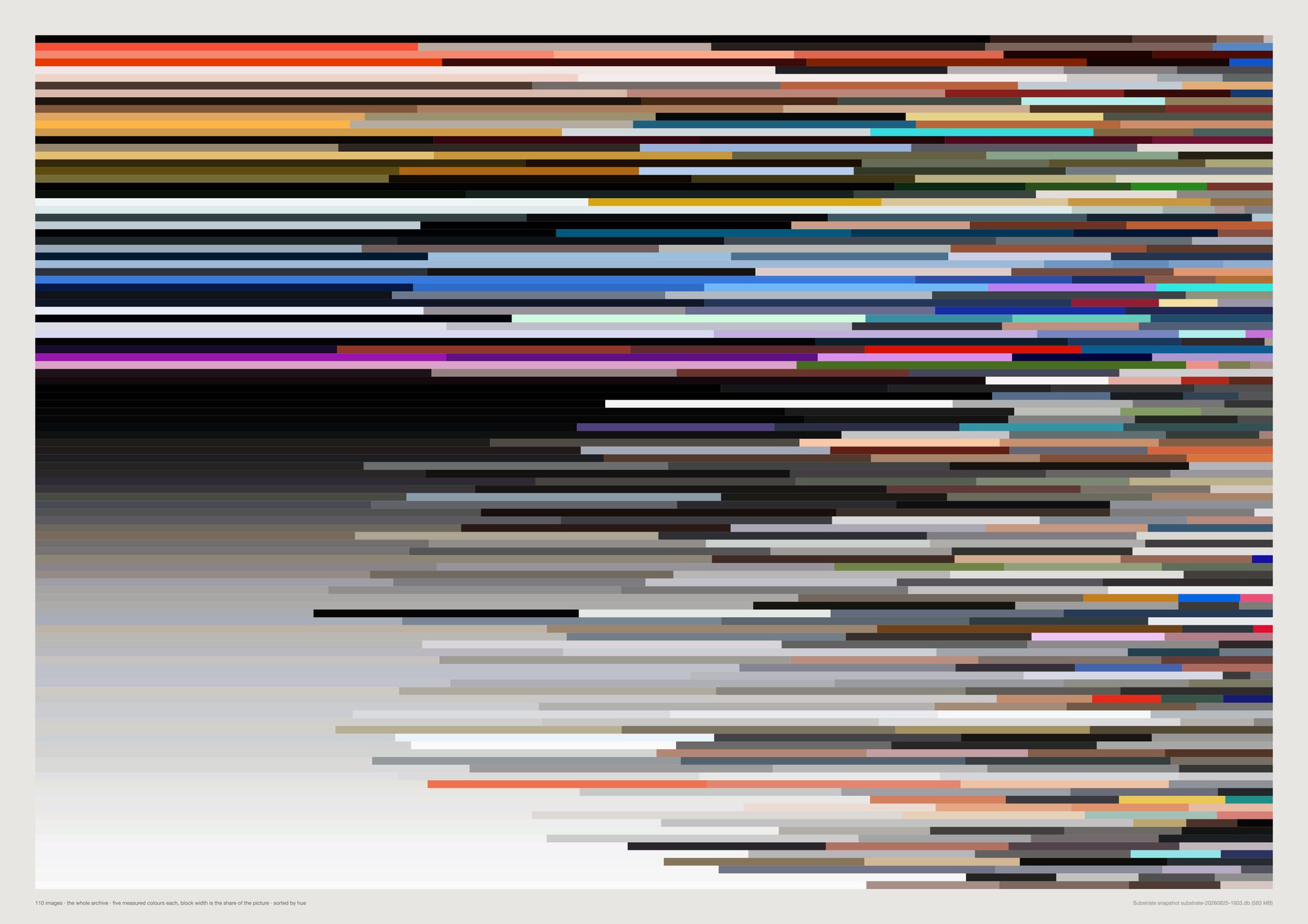
The single-colour readings elsewhere on this page are the weakest measurement in the project. This is the honest version: the dominant block is neutral in 66% of rows, and that tail now has structure instead of being a grey field.
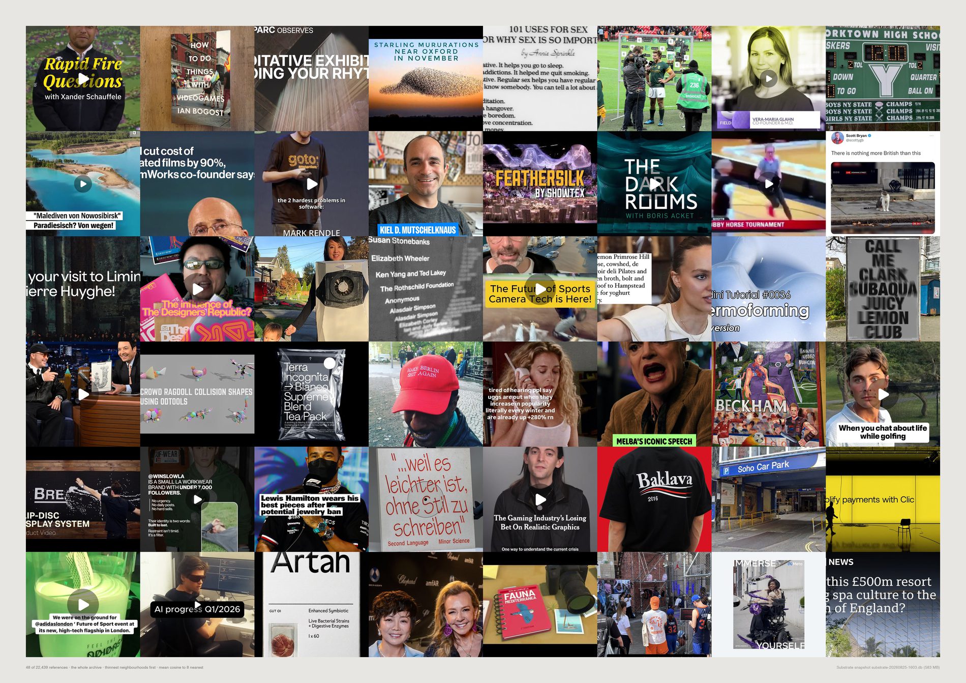
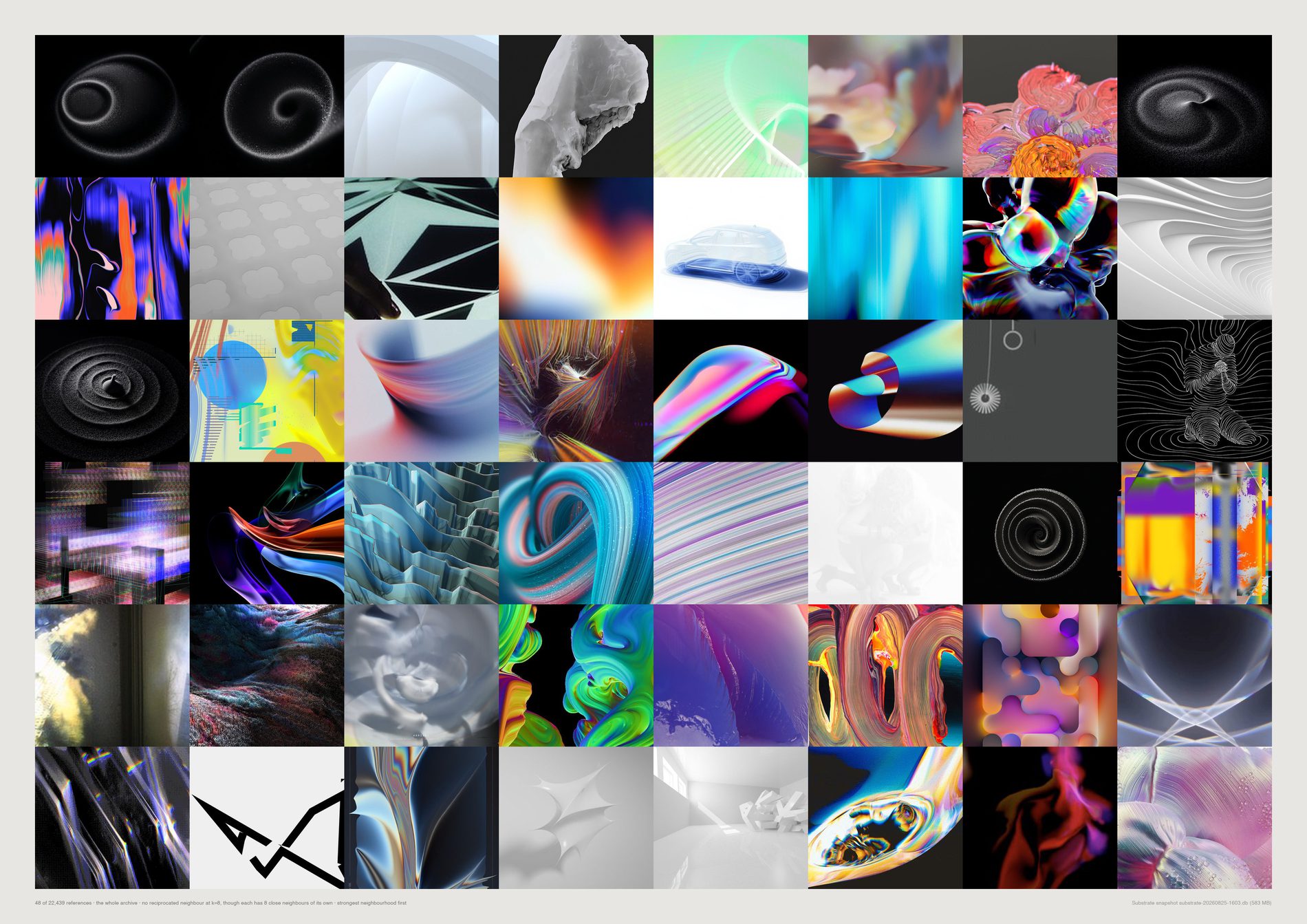
0 of the top 48 appear in both. Density-lonely images sit at cosine 0.352–0.531; mutually-lonely ones at 0.883–0.913 — they have plenty of neighbours, they are just in nobody else's top eight.
4,504 references (25.7%) have no reciprocated edge.
Only 2,018 (11.5%) are in nobody's top eight at all. A forecaster's product is the cluster, so the singular is exactly what a forecast discards — and an archive keeps it.
The density half is still retracted. The evidence filter improved this sheet without fixing it — see the correction for what it caught and what it still misses. The mutual half stands.
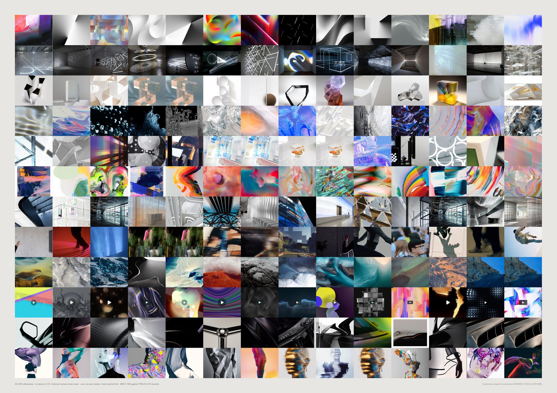
The two partitions are related but largely different. Ten of the twelve clusters are a mixture, with no board holding more than 38% of one. There really are groupings here that nobody ever named — gradients, light installations, glass objects, night photography.
One cluster is not like the others. A single cluster of 1,329 references is 78% Instagram, and that is a source artefact rather than a discovered group: Instagram captures share a crop, a compression and a graphic register before they share anything about taste. It is the same failure mode as the loners sheet, visible here as one clean band. The median purity of 0.12 is what the other eleven look like.
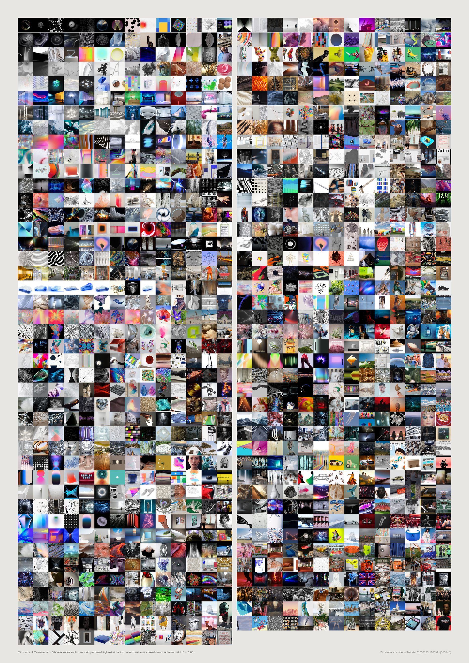
Loosest: Culture 0.713 — and, uncomfortably, the two biggest pitch boards in the archive, P062 Dystopia987 at 0.723 and P332 NikeTown London 2027 at 0.736, with Diesel Digital Nature SS16 at 0.726 and X Activist Aesthetics at 0.728 between them. Tightest: X future minimalism 0.843 and Parametricism + Materials 0.842. Correlation with log board size is only −0.11, so this is not simply a big-boards-are-messy effect. Images are sampled along each board's own centrality ranking rather than taken from its head, so a loose board actually looks loose.
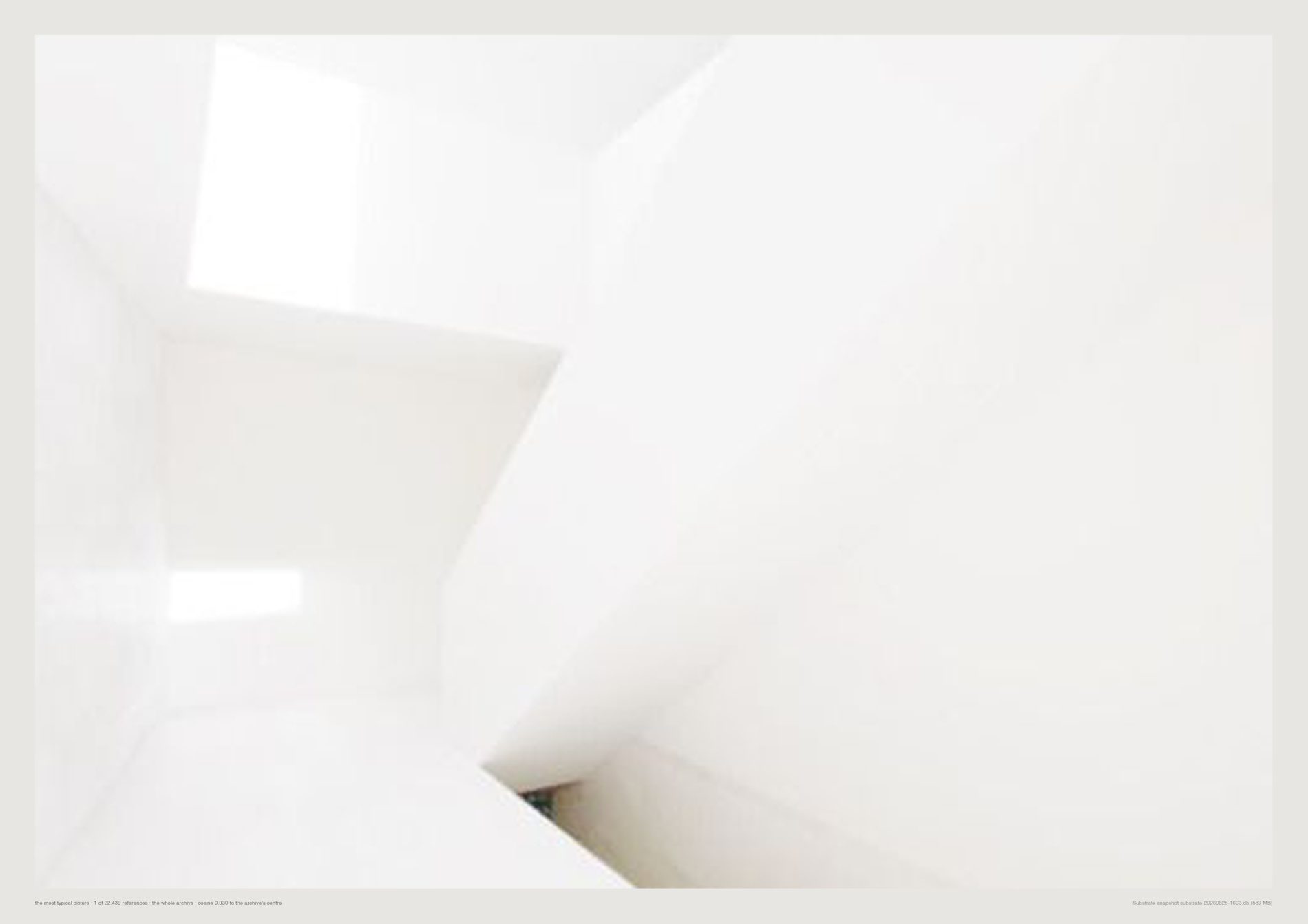
Flattering and slightly damning at once, which is why it earns a plate rather than a caption.

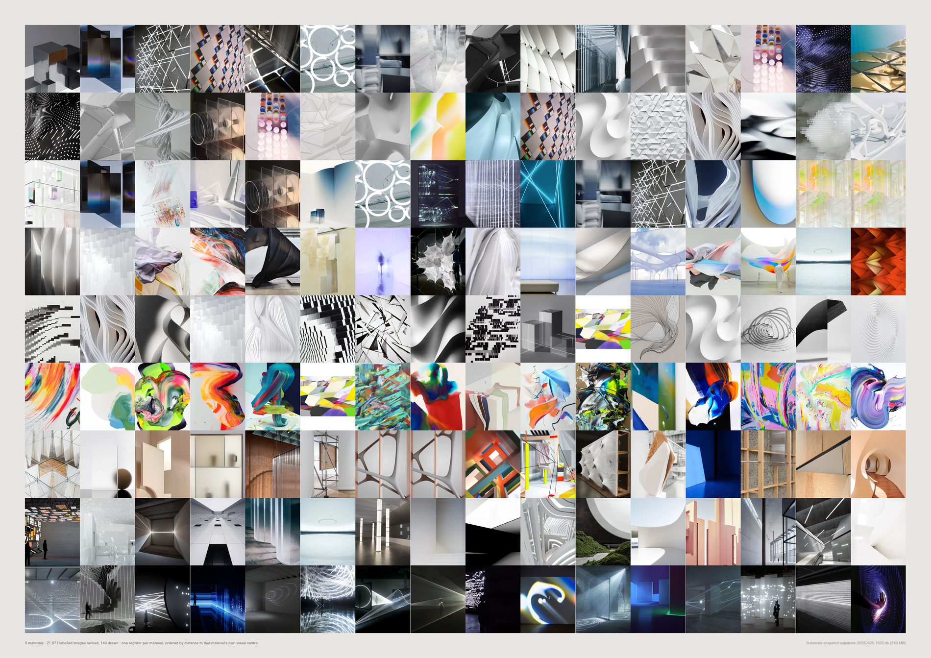
Materials are not exclusive — an image can appear in three rows. Paint, fabric and light are unmistakable at a glance; metal and glass overlap, which is honest rather than a fault of the sheet.
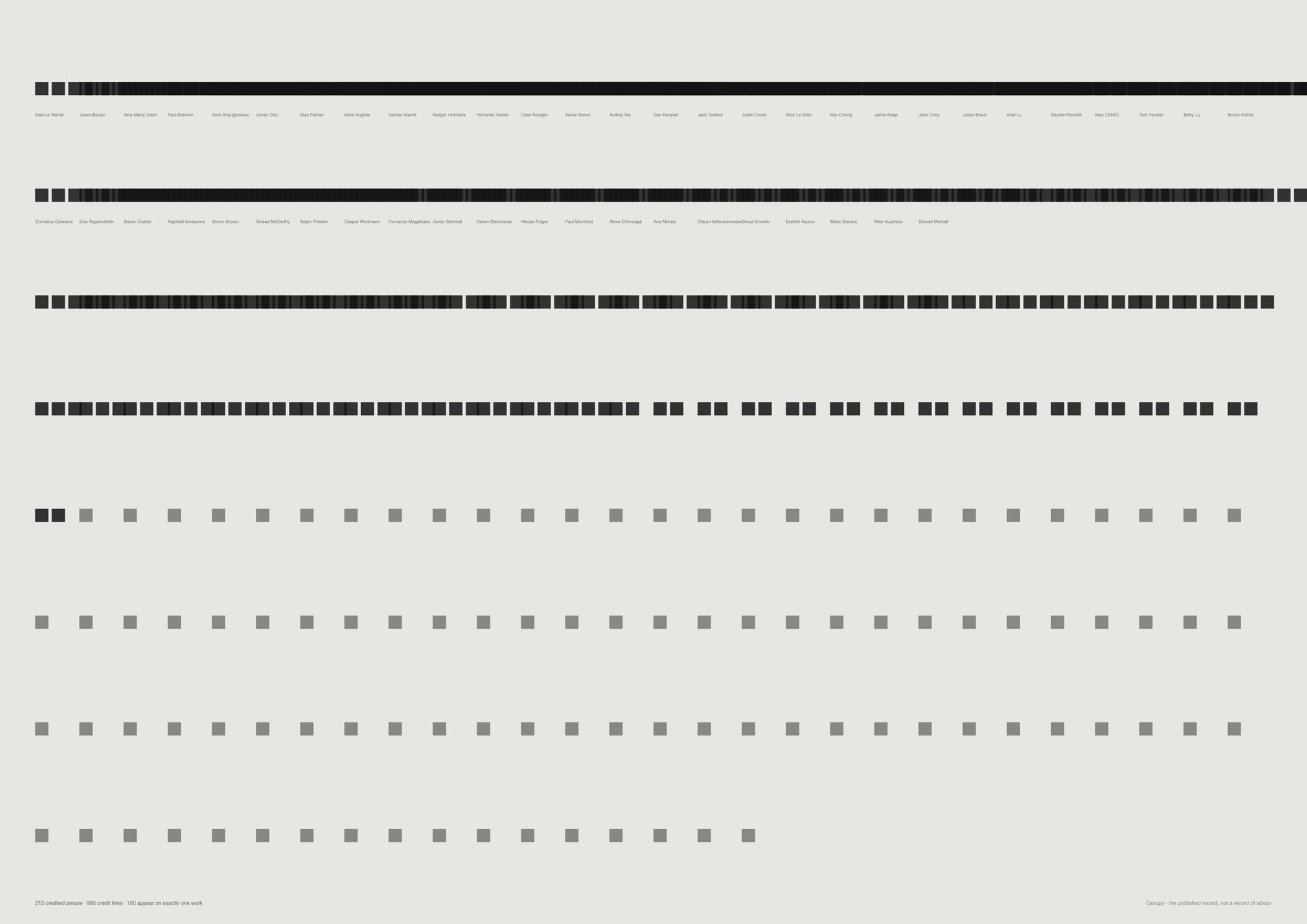
100 of 213 credited people appear on exactly one piece of work. Just under half of everyone named in the published record passed through once. The median person is credited on two.
That is not a scandal — it is how a studio of this kind works, with specialists, freelancers and people who were there for one job.
But it is invisible in every other view on this page.
Why a list and not a network. The obvious move is a co-credit graph and it fails: at an edge weight of three or more it collapses to a single component containing all 96 remaining people at density 0.158. Thresholding shrinks it without ever splitting it, because a studio is not a social network — almost everyone has worked with almost everyone. The distribution carries the finding; a hairball would not.
And credits are a publishing artefact, not a record of labour. They reflect who was listed on a case study written up later, sometimes by someone who was not there. Read it as who the studio names.
python3 src/viz/credited.py --counts
python3 src/viz/credited.py --page a2l --flat
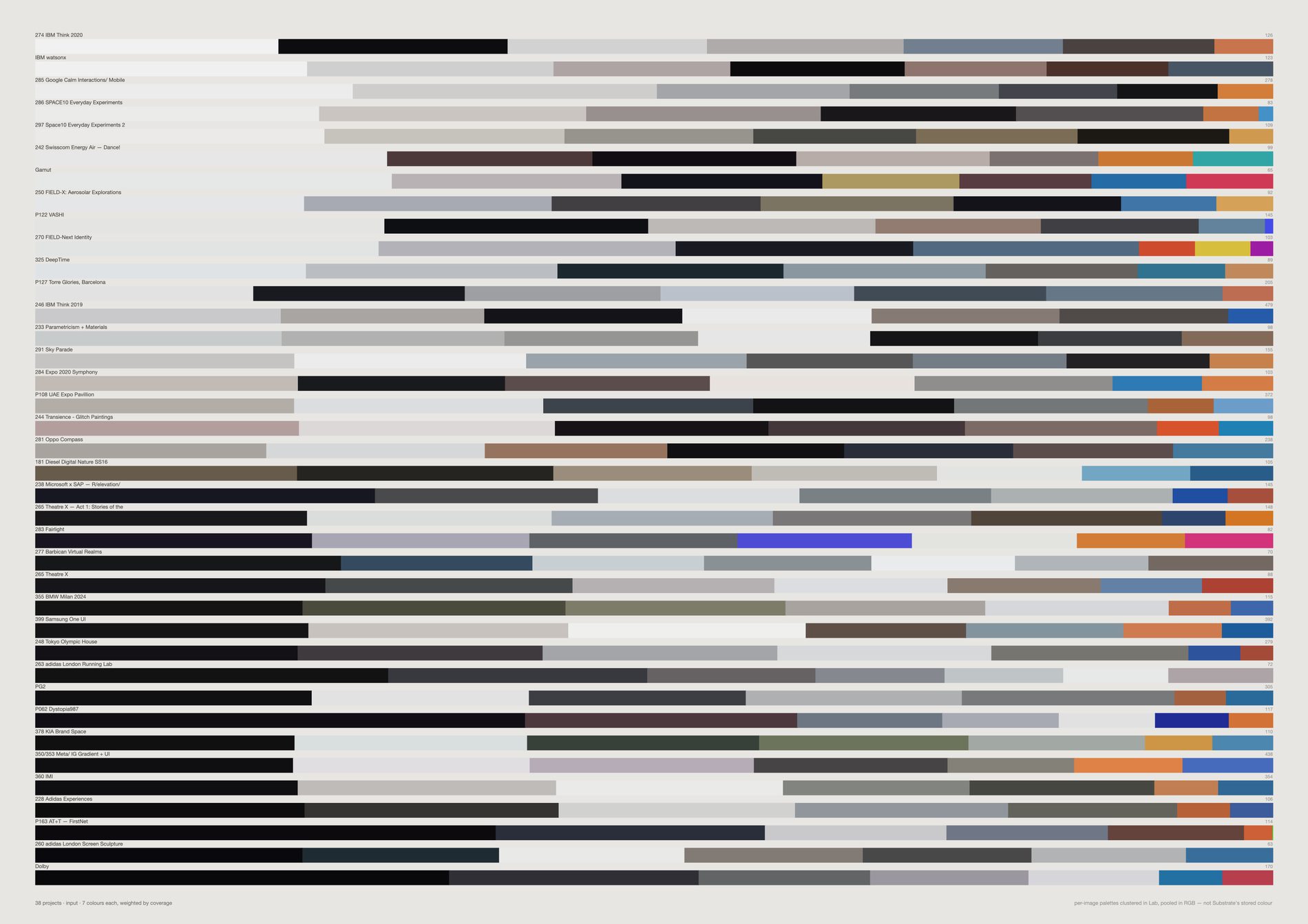
The weighting is what separates this from a mood board. A mood board shows the colours someone noticed; this shows the colours that were actually there, in proportion. Read down the sheet and the studio's range is legible in one pass — Lucient.space, IMI and Samsung One UI at the pale end, AT&T FirstNet, Dolby and adidas London Screen Sculpture at the dark, each carrying one chromatic accent at its right edge.
Three different measurements, never mixed. The per-image palettes are weighted k-means in CIE Lab. Pooling them into a row clusters in RGB, which is cruder but is grouping already-clustered representatives rather than raw pixels. Substrate's own dominant_color is a third method again. --side both puts collected against published, which is the more honest comparison.
python3 src/viz/brand_palettes.py --by project --sort lightness --k 7
python3 src/viz/brand_palettes.py --side both
The loners sheet claimed to show what nothing else in the archive resembles — a taste frontier. Checked against the whole archive, the 300 most isolated references are:
made: typography 6.5× over-represented · subject: graphic 4.6× · media_type: link 4.0× · subject: typography 4.0× · media_type: social 3.0×
while render and pin are under-represented at 0.5×.
An image with words in it sits far from photographs in CLIP space because it is a different kind of thing, not because the eye went somewhere unusual. The measure was finding a media-type artefact.
The sheet stays up because the retraction is more useful than the claim was.
The fix, and its cost. src/aesthetic.py defines what counts as evidence about taste and src/pool.py is the one place every sheet asks; together they exclude non-aesthetic media types and images the vision model called typography or diagram, while protecting the 106 live pins FIELD deliberately re-saved from its own earlier save. That removes 5,649 of 33,455 references (22%), and a strict version removes 38%. It will also throw away real references — a poster is typography and it is also design — so the module prints the cost rather than hiding it, and deletes nothing.
Same measurement, re-run over the filtered pool. Two of the three worst artefacts are gone:
made: typography at 6.5× and media_type: link at 4.0× no longer appear at all · subject: typography falls from 4.0× to 2.2×
But two barely moved:
subject: graphic 4.2× (was 4.6×) · media_type: social 2.9× (was 3.0×)
An Instagram video still with a headline burnt into it is not a link, and the vision model does not call it typography — it calls it a photograph of a person. So the filter never sees it, and it still lands at the frontier for exactly the reason the original 300 did: it is a different kind of object from a photograph. Of the 48 cells the density sheet actually draws, 25 are Instagram posts and 21 carry text by the vision record, against a 14% baseline across the pool.
The frontier claim therefore stays retracted for --mode density. It stands for --mode mutual, which is 33 pins out of 48 and sits below the text baseline — the two modes disagree completely, and only one of them was ever measuring the archive's edge.
Fixing this properly needs a text-in-image detector rather than a media-type rule, which is a different pass over 23,000 images and is not done. Stated here rather than left for a reader to notice.
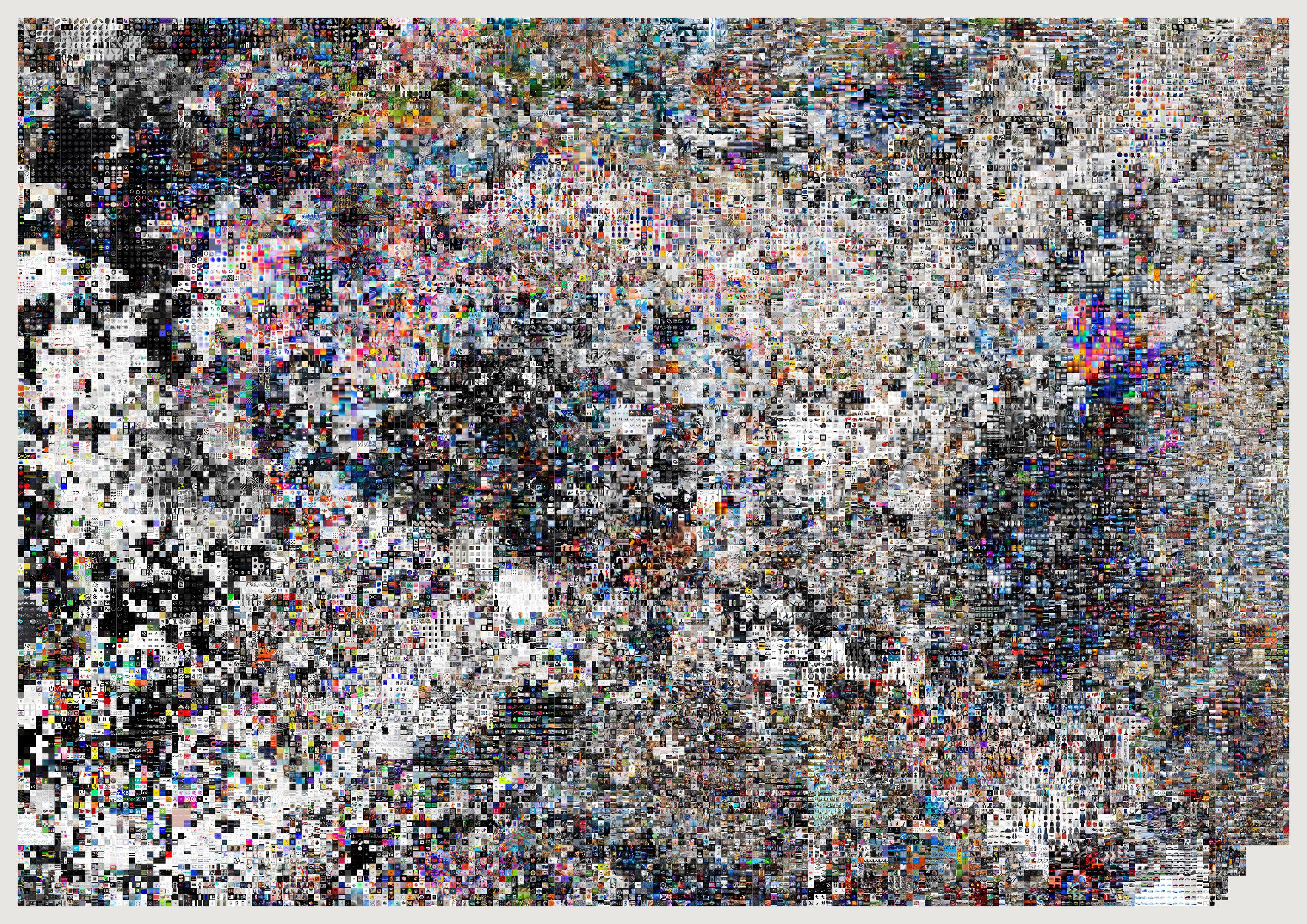
The other atlases draw the evidence pool, 21,491 references. This draws everything. The pool exists because a sheet about taste should not be half screenshots and duplicate saves; this sheet is not about taste, it is about size, so the filter comes off and the near-duplicates stay in. A studio that saved the same picture twice did save it twice.
29,783 of 33,457, and the shortfall is not a filter. An image can only be placed if it has a CLIP vector and a cached file; the 3,674 that have neither are mostly notes and articles carrying no usable picture. So this is the whole archive as far as the archive can be drawn, which is a different sentence from “the whole archive” and the caption says the first one.
python3 src/viz/atlas.py --everything --max 40000 --page 1189x841 --dpi 200 --out atlas-archive
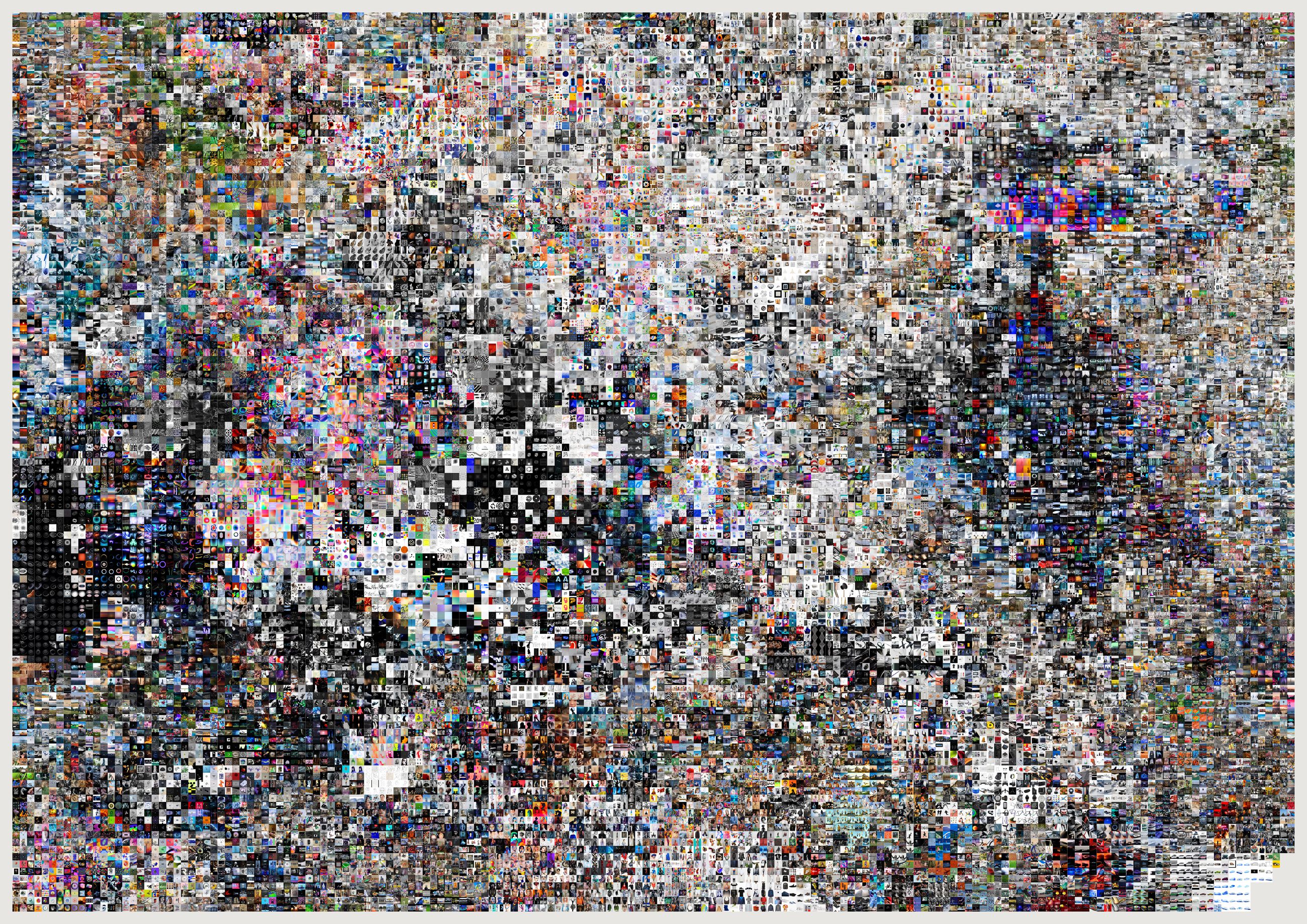
Above a certain density individual marks stop being pictures and become tone. That is the same reason Graphcore's compute-graph renderings work at 115 million edges and a 25,000-node network does not: below roughly twenty elements you read structure, above roughly ten million you read texture, and the middle is where archive visualisations go to die. This sheet is deliberately pushed toward the texture end.
Derived edges make hairballs; deliberate edges make pictures.
The artist graph does not exist and is not derivable — 7 co-channel edges at weight three or more, zero at five.
The co-credit graph is real but at weight three collapses into a single component of all 96 remaining people at density 0.158; thresholding shrinks it without splitting it, because almost everyone in a studio has worked with almost everyone.
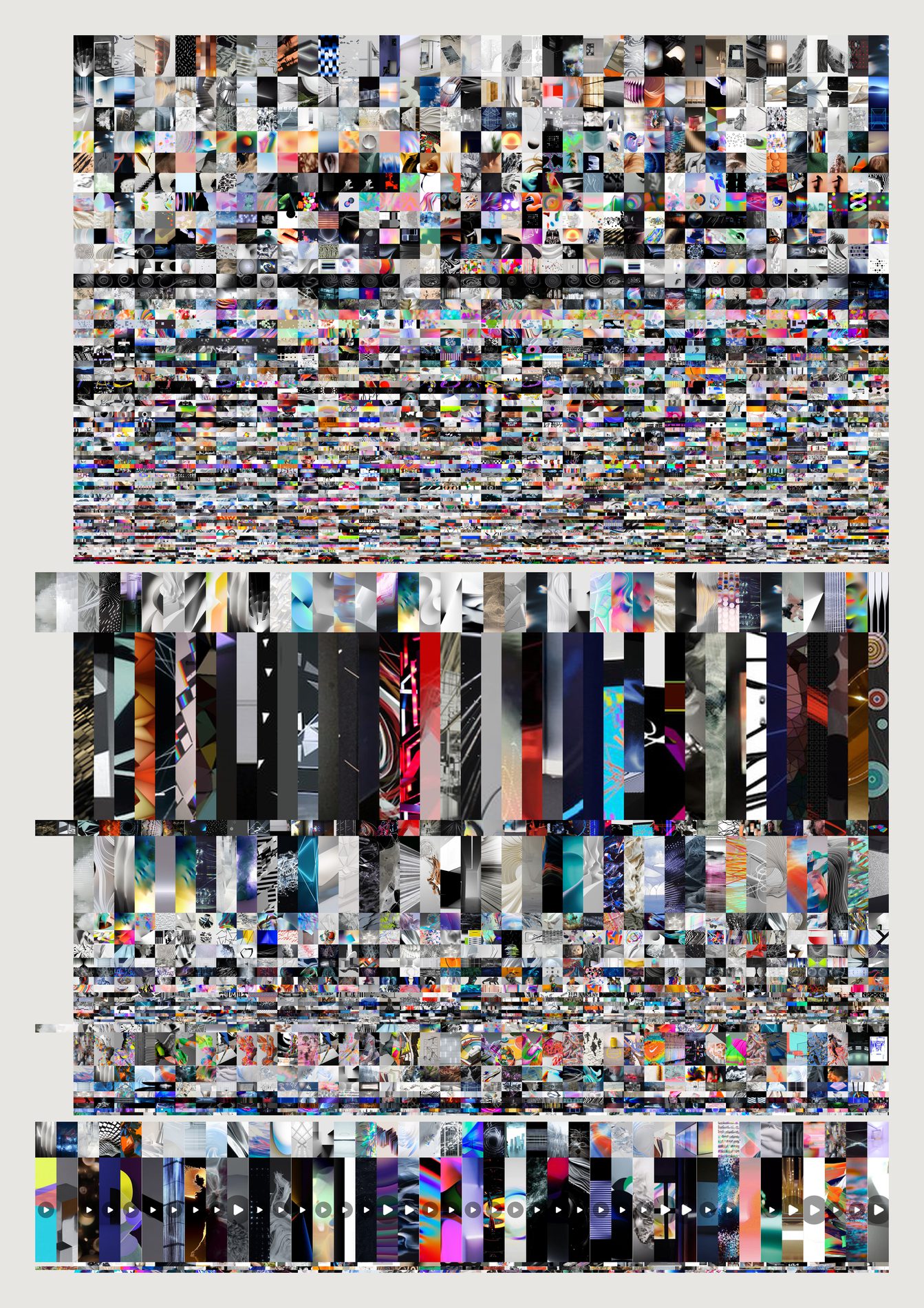
The channel tree is the one structure here whose edges were put there on purpose. Someone decided Explorations belongs under Aesthetics. Depth is containment and height is share — both sayable in a sentence, which is the test a position has to pass.
The first attempt failed and the fix is visible. Drawing every band full width made a handsome texture in which the hierarchy vanished entirely. Each level is now inset from its parent so containment reads without a label, and each image is cropped to its cell's aspect before resizing — resizing straight into a thin band smears every picture into a streak that looks like a rendering fault rather than like the archive.
And height is count, not importance. The largest band is Creative Applications, a subscription feed rather than a decision anyone made about taste. That is worth seeing rather than correcting away.
python3 src/viz/tree_images.py --depth 2 --min 60 --page a2 --dpi 200
python3 src/publish.py mehretu-dense
# python3 src/viz/mehretu.py --n 9000 --k 6 --mark-scale 1.6 --flags 6.9 --page a2l --dpi 200 --out mehretu-dense
She is in the archive, which is why these exist. Fifteen references name Julie Mehretu: two saved in 2012, the archive's first year, into Data and Form; eleven in 2018 across two real jobs, 238 Microsoft × SAP and Aeternity — Crypto Drone Painting. The studio was looking at her, and using her, six years before any of this. The two most recent were saved on 25 August 2026, and they are two of these sheets — captured back into the archive by the Basecamp archivist, filed under Human First.
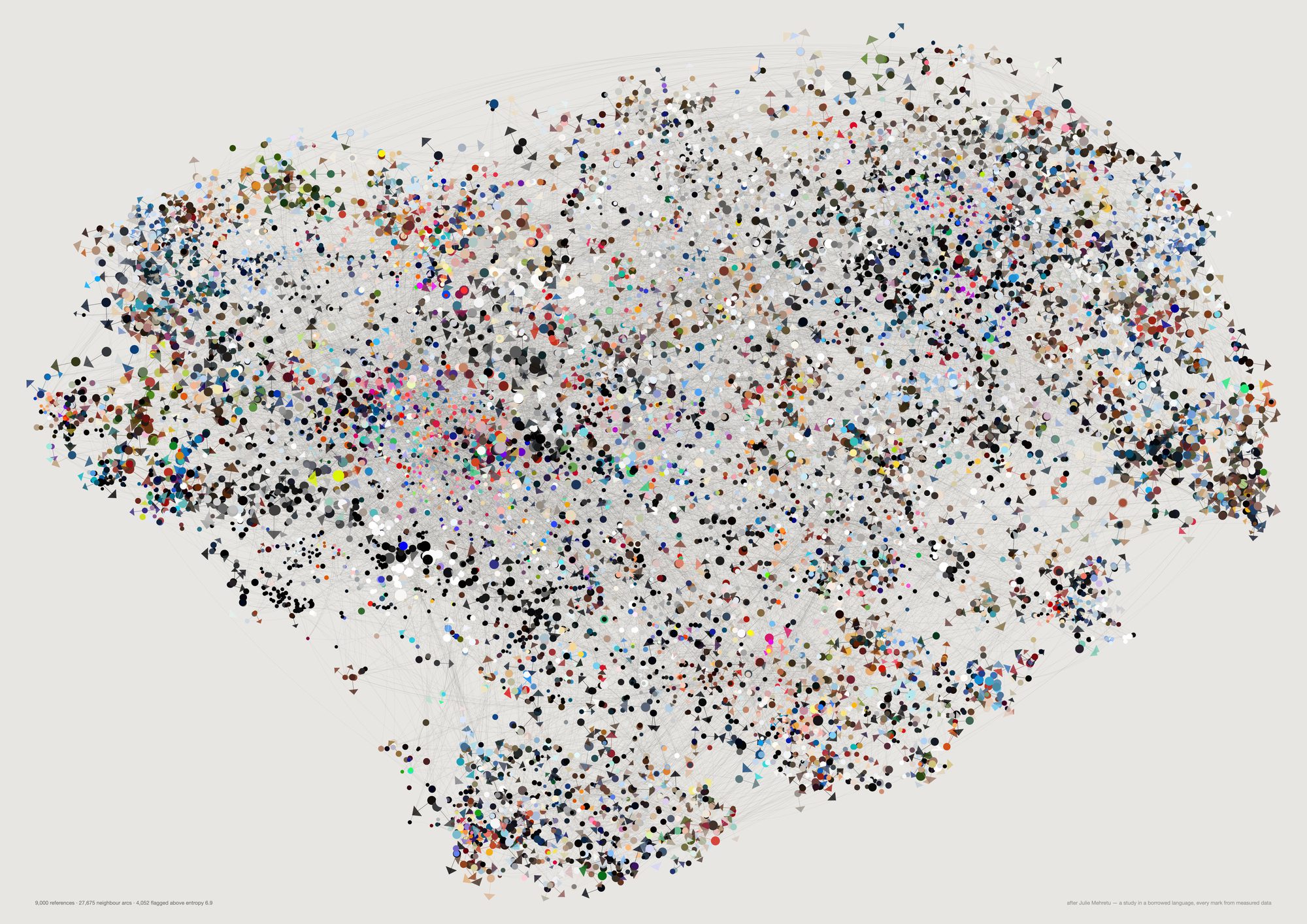
Position is the t-SNE coordinate, so two marks near each other are two references that look alike. The line-work is the nearest-neighbour graph — dense knots are territory the studio returned to, open ground is territory it never occupied. Colour is each reference's measured vivid reading, mark size is edge density, and the flags fall only on the most visually complex references, so the storm gathers where the archive is busiest.
This is pastiche of a living artist and should carry her name wherever it appears. Julie Mehretu is in this archive — thirteen references, the oldest pinned 2012-03-30 — which is why she came to mind, and is also why the piece needs attribution rather than quiet absorption. It is a study, not a form FIELD invented. Three further studies follow it below, with their controls.
And the density flatters. A nearest-neighbour graph over thousands of points produces a beautiful mesh regardless of what the underlying data is. Draw random vectors this way and it still looks like weather. The form here is borrowed and the content is honest, which is an easy combination to misread — the resemblance is not a claim that the archive is Mehretu-like.
python3 src/viz/mehretu.py --n 9000 --k 6 --mark-scale 1.6 --flags 6.9 --page a2l --dpi 200 --out mehretu-dense
One study turned into a family. The first sheet is above; everything here is the same archive redrawn, with each version's own control printed beside it rather than in a footnote. Read the framing first — the controls are the reason this section exists.
This is pastiche of a living artist, and in print it goes with her name on it. Julie Mehretu is in this archive — thirteen references, the oldest pinned 2012-03-30 — which is why she came to mind, and it is also why the piece needs attribution rather than quiet absorption. It is a study in a borrowed language, not a form FIELD invented. The closer the resemblance gets the more that matters, and every sheet below is closer than the one above it.
The second study shuffled every measurement across the real positions and re-rendered through the same code path, same parameters, same everything else.
Random vectors are obviously distinguishable, and that is the good news. t-SNE over gaussian noise gives a radially symmetric hairball — no lobes, no islands, no bays of empty paper — and every plan block collapses to the same page-sized rectangle, because a channel whose members are scattered at random has no centroid worth drawing. So the layout is carrying real information.
Shuffled real measurements are very nearly not distinguishable, and that is the finding. Keep every true position and permute only the readings across them, and at reading distance it is the same picture. Measured as mean RGB distance to twelve page-neighbours, the real sheet is 10% more colour-clustered than chance on vivid and 22% on brightness_med. Ten per cent is not much to hang a picture on. The substrate carries the information and the storm carries almost none of it — position, density and the channel plan do the work, while the per-mark bindings are true, are measured, and are individually invisible once there are nine thousand of them on one page.
The scribbles came out because Marcus did not like them, so the obvious hypothesis was that they were the noise hiding the signal. They were not. Restricting the same test to the marks actually drawn in colour makes the gap narrower, not wider: 9.2% on the second study's colour set and 9.4% on the third's, against 11.3% for all marks. Taking the scribbles out was the right taste call and it is not the evidence.
What widened was straightening. This sheet is mostly made of direction, and direction is what the second study never measured. At its 55° turn, the correlation between mark directions at 6% of the page width was 0.0058 real against 0.0025 shuffled — both flat zero, so the storm was being combed by a current that was statistically invisible on the page. Turn the residual down to 16° and the same statistic is 0.181 against 0.059, a 3.1× gap that holds at about 2.7× anywhere below 30° of turn. The picture agrees with the number: the third study's shuffle is tellable from the real sheet at a glance, where the second study's needed a loupe and a table.
| Shuffle control, n=9,000, 24 permutations, 12 page-neighbours | real | shuffled | gap |
|---|---|---|---|
| A · vivid RGB, all marks | 162.9 | 181.4 | 11.3% |
| B · brightness_med, the flow scalar | 0.2477 | 0.3179 | 28.3% |
| C · vivid RGB, second study's colour set (q0.62) | 170.9 | 186.6 | 9.2% |
| C′ · vivid RGB, third study's colour set (q0.45) | 167.4 | 183.2 | 9.4% |
| D · flow-field variance | 0.004768 | 0.0002452 | 19× |
| E · mark direction, 12 neighbours, turn 55° | 0.4362 | 0.2779 | 57% |
| E′ · the same, turn 16° | 0.8358 | 0.7820 | 6.9% |
| F · current reach at 6% of the page, turn 55° | 0.005765 | 0.002548 | both ≈ 0 |
| F′ · the same, turn 16° | 0.1808 | 0.05872 | 3.1× |
Both earlier controls turned on statistics a viewer would have to be told about. The fourth study makes the mark vocabulary carry the confidence instead — a sliver only where the twelve nearest marks agree on an axis, a dot where they do not — so the statistic becomes which mark got drawn. Share of references earning a direction: 66.5% real against 51.5% shuffled at n=9,000, a 15-point gap, and 54.8% against 37.1% at n=4,200. It holds across the threshold (+12.6 points at 0.80, +19.5 at 0.90), and the control sheet is visibly stippled where the real one is combed. Statistics A to F reproduce the table below to four significant figures at n=9,000, which is the check that this is the same metric and not a new one wearing the old name.
Two negatives that come with it. Reducing the grey moved A, B and C not at all — it is a decision about looking, not a gain in evidence. And the bold-set clustering statistic does not discriminate between bolding by evidence and bolding by pigment (30.4% against 31.2% tighter than their nulls), so it says both bold sets are spatially structured and nothing about which rule is better.
A permuted archive still produces a flow grid, but its cell means are sampling noise, and blurring noise leaves almost nothing behind. 19× is not a marginal result.
E is local. At a low turn it saturates, because blur any field enough and the immediate neighbours agree whatever is underneath. F is the one that matches what a person standing in front of the sheet sees: how far the agreement reaches.
The second study quoted A and B as 10% and 22% because it expressed the gap against the shuffled value; the report here expresses it against the real one, giving 11.3% and 28.3%. Same numbers, same finding, and the arithmetic is checkable from the two columns beside them.
Two things the control cannot rescue. The currents reach about 6% of the page and no further — at 18% and 35% the correlation is back at zero, so these are local weather systems and not a composition, and the composition is still the t-SNE layout doing the work. And a 3× gap on a directional statistic is a gap a viewer could see once told, not one they would have noticed unprompted. These sheets should hang next to the plain ones rather than instead of them, and the caption on the wall should say study, not finding.
python3 src/viz/mehretu3.py --n 9000 --report
The second study. Marcus, on the first: “these are just dots.” Raising the count did not fix that, because the problem was never density — every mark sat in the same size register, pointed in a direction chosen by a golden angle, and floated on empty paper with no substrate underneath. This version builds the sheet in explicit strata, and binds every one of them to something measured: the channel tree as an architectural plan, veils averaged from real palettes, a flow field of brightness_med whose iso-lines every directional mark runs along, and a turbulence term that turns each mark off the current by its own residual. Her ground is warm cream, so these three pass --paper "#efe9dd".
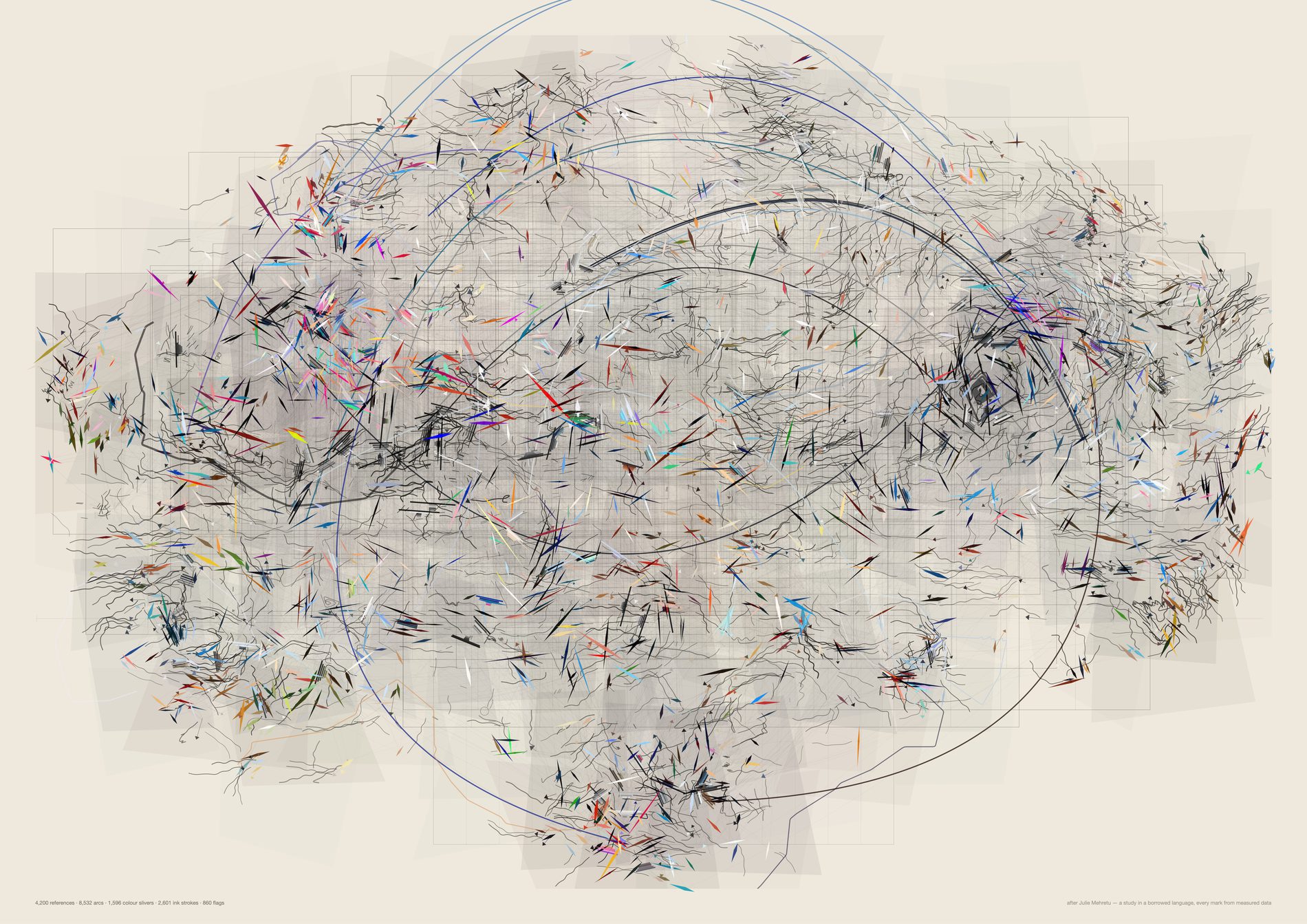
The saturation gate is what produces the division of labour: every reference below it becomes ink — a scribble traced along the flow, segment count from entropy, curl amplitude from edge density, darkness from local density — and every reference above it becomes a flat tapered lozenge in its own measured vivid, length from its aspect ratio, width from its edge density. At this count you can still see the plan under the storm.
The plan is the one structure in the archive a human authored. 309 nodes three levels deep, each channel drawn centred on the t-SNE centroid of its own members and sized to one standard deviation of their spread, so a tight channel is a small box and a diffuse one is a large one. Everything else on the sheet is derived.
python3 src/viz/mehretu2.py --n 4200 --k 4 --bands 240 --gestures 20 --plan-min 25 --page a2l --dpi 300 --paper "#efe9dd" --out mehretu2-open
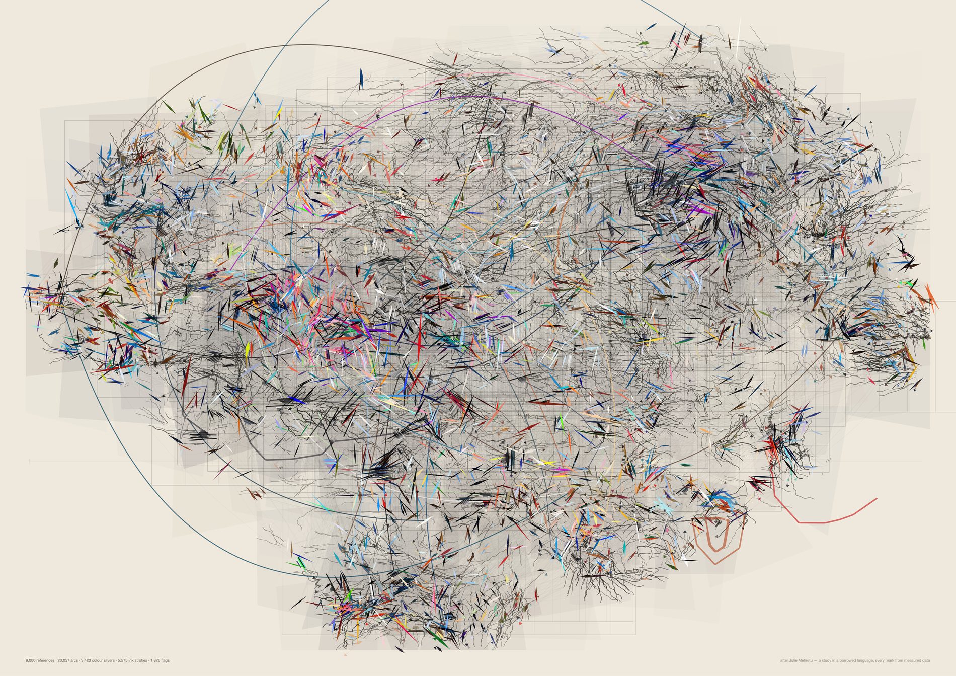
Eleven layers, bottom to top: the plan, the section rules, the veils, the kNN line-work, the long gestures, the ink storms, the colour slivers, the palette bands, the flags, the punctuation, and the returns — a fine open ring on each of the 106 deliberate re-saves, the only mark here that is about an act rather than an image. The near-black knots and the near-white passages come from the density field; nothing is thinned by hand.
The turbulence term is doing more than it looks like. Each mark is turned off the current by how far its own reading sits from the mean of the neighbourhood it landed in, clipped to one standard deviation and scaled to at most 55°. So the crossing marks are the local misfits, and they are the only reason this storm has any turbulence in it at all. The control found that 55° is also what makes the current statistically invisible.
python3 src/viz/mehretu2.py --n 9000 --page a2l --dpi 300 --paper "#efe9dd"
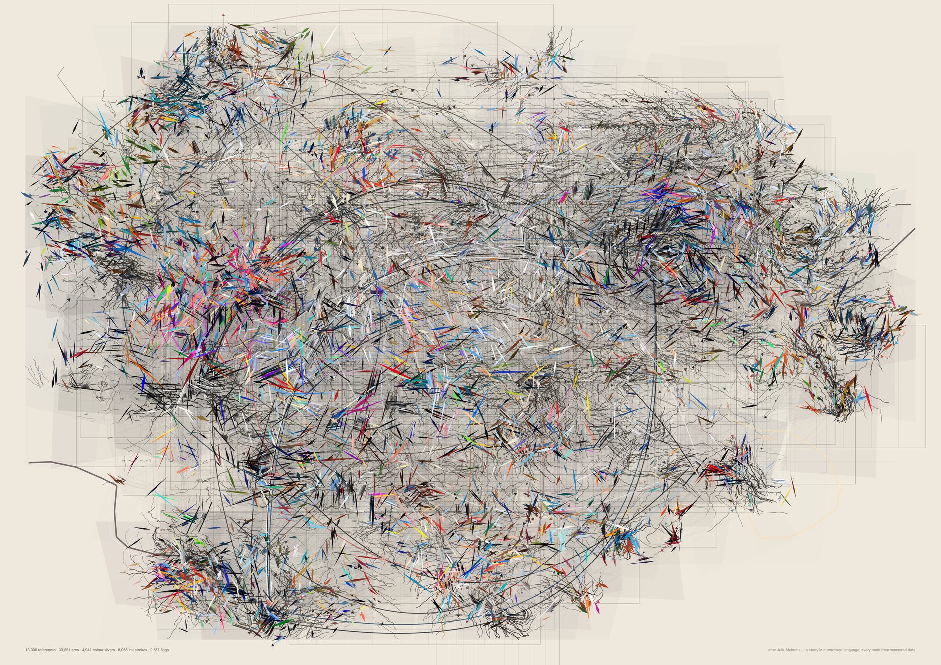
Past about nine thousand the storm begins closing over the plan, and what is left to look at is the bays — the passages of near-white paper the archive never occupied.
The whole pool exists but has no proof. A 21,491-reference render with 41,454 arcs is written with --no-proof: the SVG is complete and is the file that would go to print, but this box has no rsvg-convert, so proofs go through macOS qlmanage, which parses a 5.5 MB SVG happily and hangs indefinitely on an 11 MB one at any dpi. 13,000 is the densest variant that proofs here, and brew install librsvg is the fix.
python3 src/viz/mehretu2.py --n 13000 --k 5 --bands 620 --gestures 32 --page a2l --dpi 260 --paper "#efe9dd" --out mehretu2-dense
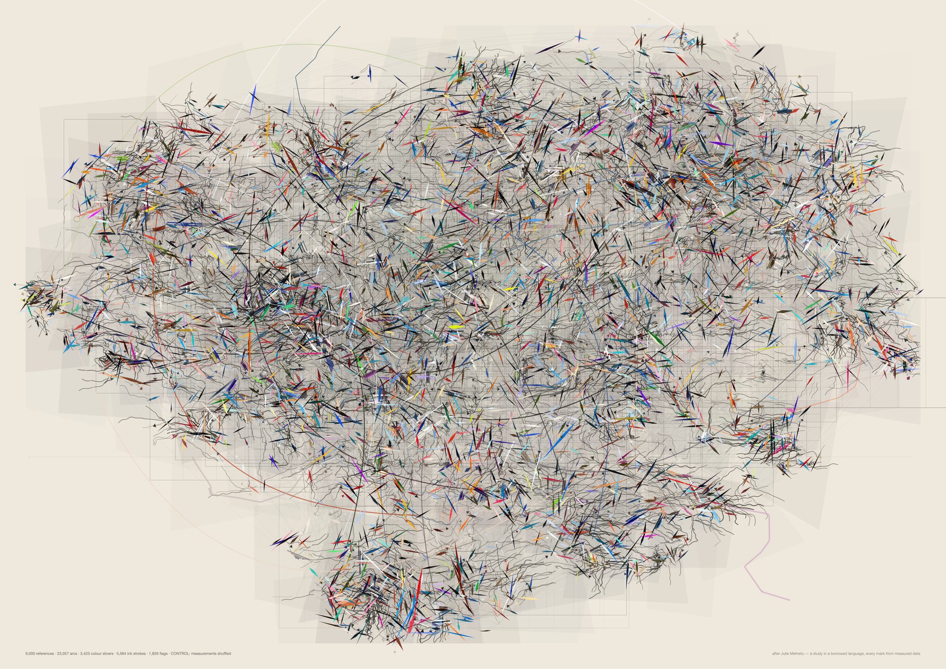
Set this beside the real sheet and try to tell them apart. Same currents, same knots, same colour weight. The difference survives only on close inspection, as the loss of local colour patches, and when measured it is 10% on vivid and 22% on brightness_med. Every mark on the real sheet is bound to a real reading, and that is what nine thousand true bindings on one page look like against chance.
This sheet is here to be compared, not admired. It is drawn at 130dpi rather than 300 because it is a null and not a print file. The reason it is on the page at all is that a study which looks like evidence should have to show what its own noise looks like, at the same size, in the same section.
python3 src/viz/mehretu2.py --n 9000 --control shuffle --page a2l --dpi 130 --paper "#efe9dd"
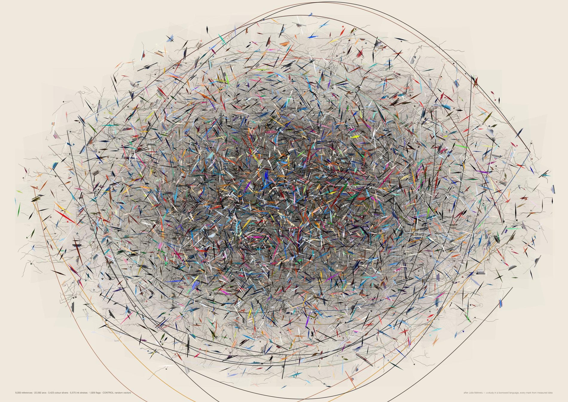
t-SNE over gaussian noise is a radially symmetric disc with a uniformly dense core: no lobes, no islands, no bays of empty paper, no vortices. Every plan block collapses to the same page-sized rectangle, because a channel whose members are scattered at random has no centroid worth drawing. Beside the real sheet this reads as a hairball rather than as weather, and that is the evidence that the layout is carrying the shape of the archive.
python3 src/viz/mehretu2.py --n 9000 --control random --page a2l --dpi 130 --paper "#efe9dd"
The third study, and the first made against a reading rather than an idea. Marcus, on the open version above, three notes: “remove the beige background · make the shapes less wobbly · not a fan of those curly lines, i do like the colored strokes tho.” Each is a flag rather than a rewrite, so the difference each one makes gets a sheet of its own. All six run at 4,200 references, and the wobble turned out to be four separate parameters rather than one.
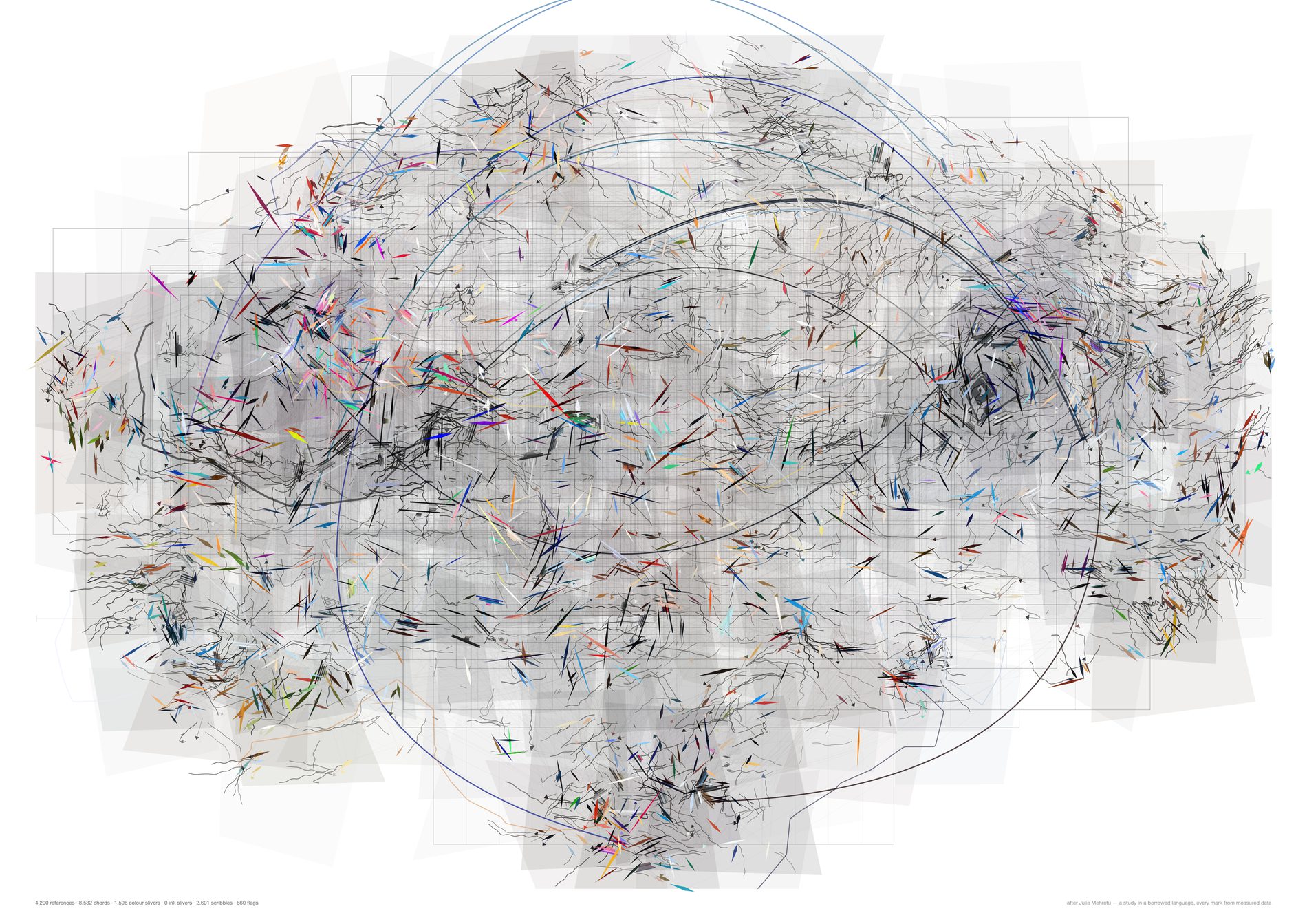
Opacity does not survive the move. A wash that reads as atmosphere on cream reads as a dirty rectangle on white, and grey line-work that sank into cream sits up off it, so the veils and the plan run at 1.4 and 1.2. Everything else here is the second study's settings exactly, which is what makes this the isolate for note one.
python3 src/viz/mehretu3.py --n 4200 --k 4 --bands 240 --gestures 20 --plan-min 25 --page a2l --dpi 300 --veil-gain 1.4 --plan-gain 1.2 --turn 55 --flow-smooth 2 --bow 0.16 --gesture-bow 1.0 --veil-jitter 0.85 --storm-q 0.62 --colour-q 0.62 --curl 1.0 --stream-steps 110 --out mehretu3-white
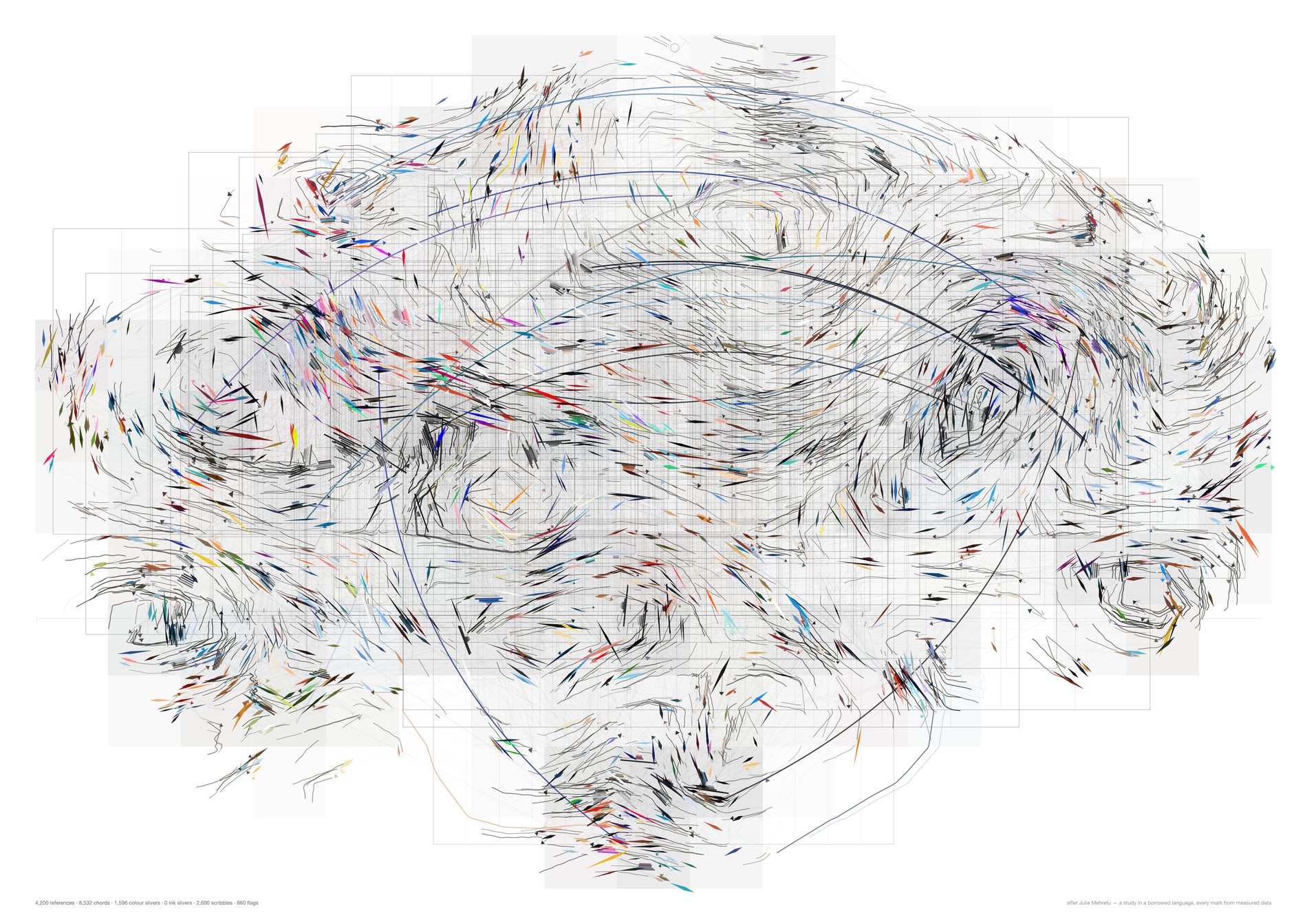
The turn, fixed at 55° in the second study and 16° here — the most consequential number on the sheet. The flow smoothing, 2 blur passes to 5, giving fewer, longer, calmer currents. The bow on the kNN line-work, 0.16 to 0, i.e. straight chords — and the bow was decoration applied to a derivation, which is the worst place to put it. The veil jitter, 0.85 of a cell to 0, i.e. rectilinear washes, and that last one is where most of the shapes being wobbly actually came from, as against the marks.
The streamlines come down too. A divergence-free field traced far enough closes into a ring, and a ring reads as a wobble. That is a property of the integration, not of the archive.
python3 src/viz/mehretu3.py --n 4200 --k 4 --bands 240 --gestures 20 --plan-min 25 --page a2l --dpi 300 --veil-gain 1.4 --plan-gain 1.2 --storm-q 0.62 --colour-q 0.62 --curl 0.35 --out mehretu3-straight
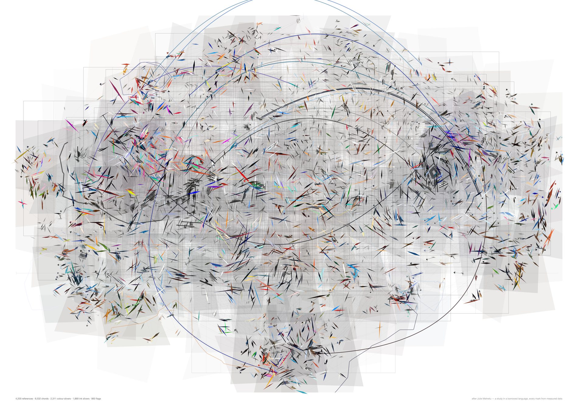
In the second study one saturation gate decided whether a reference got a scribble or a sliver, and it sent 62% of the archive into scribbles. Here there are two: --storm-q, at 0 by default so nothing scribbles, and --colour-q at 0.45, which now decides only what a sliver is made of — its own vivid above, graphite darkened by local density below, drawn finer at 0.80 length and 0.62 width so the ink carries the current without competing with the colour. The division of labour survives, in one family of marks instead of two.
This is note three with the wobble deliberately left in, so the two notes can be told apart on the page. It is not the recommended sheet; it is the isolate.
python3 src/viz/mehretu3.py --n 4200 --k 4 --bands 240 --gestures 20 --plan-min 25 --page a2l --dpi 300 --veil-gain 1.4 --plan-gain 1.2 --turn 55 --flow-smooth 2 --bow 0.16 --gesture-bow 1.0 --veil-jitter 0.85 --stream-steps 110 --out mehretu3-slivers
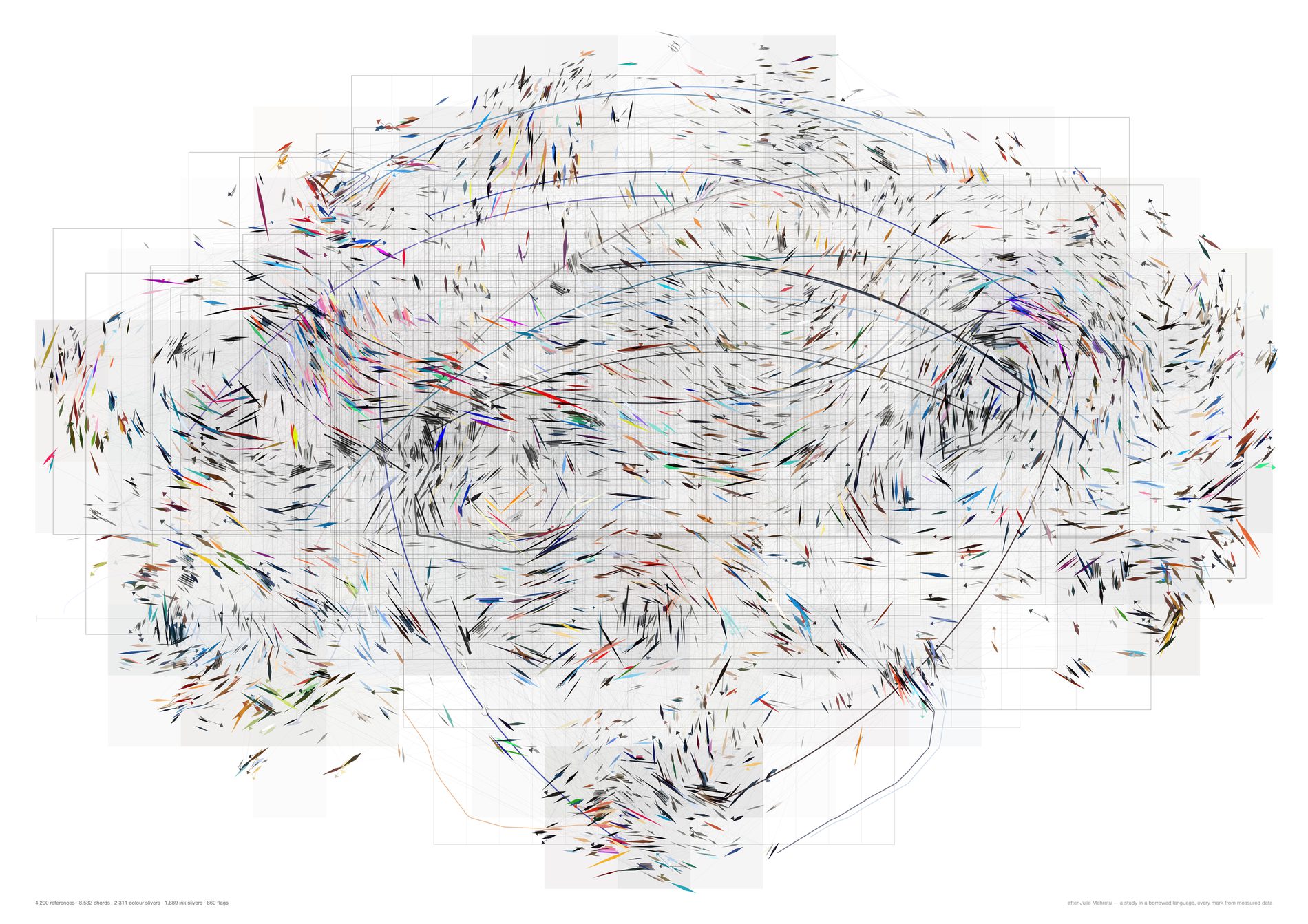
Turning the turbulence down from 55° to 16° is what makes the realness of the field visible; taking the scribbles out is what makes it legible. The measurement says the same thing bluntly: dropping the storm does not widen the gap against the null at all, and straightening the marks takes the direction correlation at 6% of the page from 0.0058 against 0.0025 — both flat zero — to 0.181 against 0.059. The full table is in the framing above.
What would make this wrong. The currents reach about 6% of the page and no further, so they are local weather systems rather than a composition, and the composition is still the t-SNE layout doing the work. A 3× gap on a directional statistic is something a viewer could see once told, not something they would notice unprompted. And the flow field is a smooth scalar: integrate any smooth scalar and you get currents, which is why the shuffle control has to be on the page beside this.
python3 src/viz/mehretu3.py --n 4200 --k 4 --bands 240 --gestures 20 --plan-min 25 --page a2l --dpi 300 --veil-gain 1.4 --plan-gain 1.2 --out mehretu3
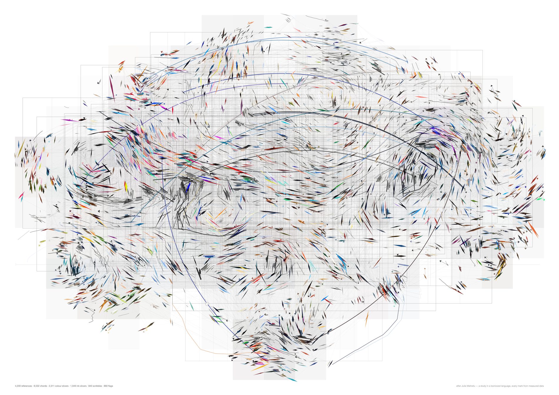
The 838 least saturated references become traces rather than lozenges — segment count from entropy, amplitude from edge density, darkness from local density, at a fifth of the second study's curl. It is the one variant where the flow field is directly legible instead of inferred from the way the slivers line up.
The layer is kept for the control's sake as much as for this sheet. Leaving the storm in the code is what lets the third study's code path draw the second study's picture, which is the only reason the two controls are comparable at all.
python3 src/viz/mehretu3.py --n 4200 --k 4 --bands 240 --gestures 20 --plan-min 25 --page a2l --dpi 300 --veil-gain 1.4 --plan-gain 1.2 --storm-q 0.20 --curl 0.25 --out mehretu3-currents
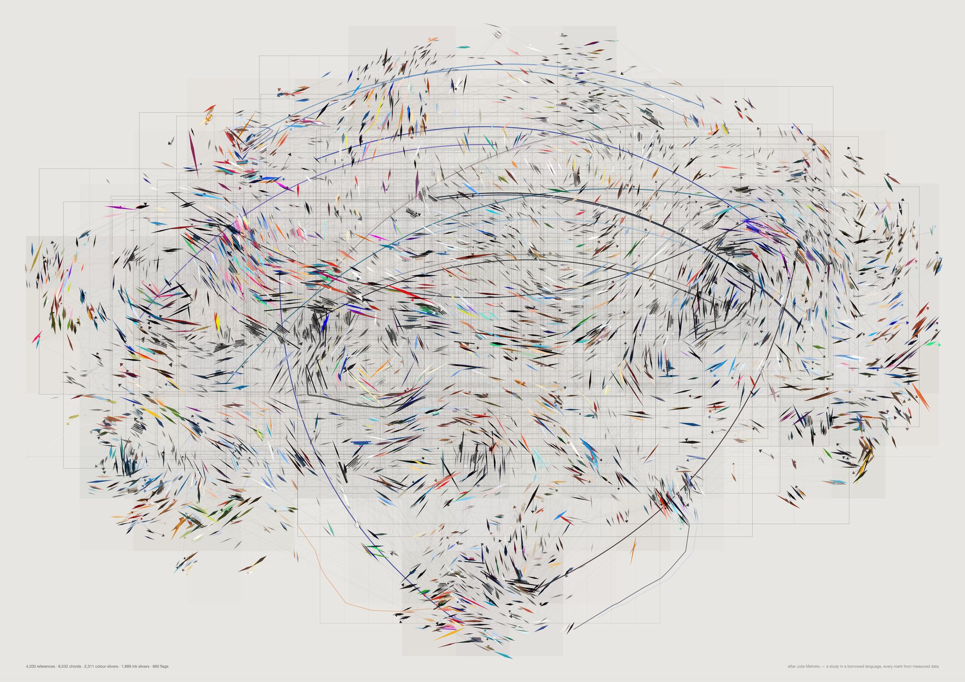
Identical marks, identical counts, no gain applied. --veil-gain and --plan-gain at 1.0 is what the second study's cream values mean, so this is the sheet that shows how much of the difference between the two studies was the paper rather than the drawing.
python3 src/viz/mehretu3.py --n 4200 --k 4 --bands 240 --gestures 20 --plan-min 25 --page a2l --dpi 300 --paper "var(--panel)" --out mehretu3-stock
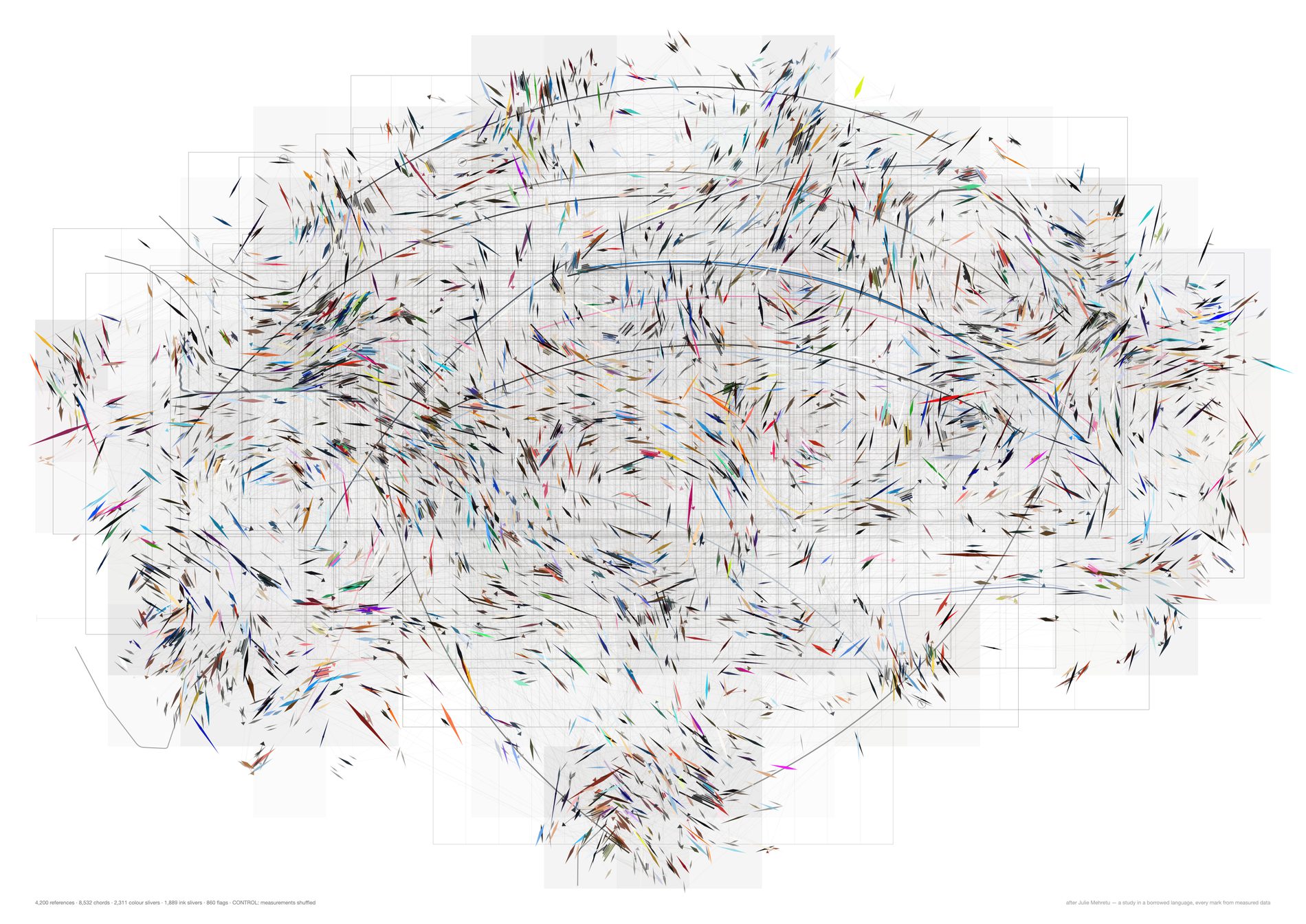
Set this beside the real sheet and the currents are simply absent. That is the strongest claim these sheets have: not that the drawing is beautiful, but that its own null is now visibly a different picture, where the second study's null needed a loupe and a table to separate.
It is still only the direction that separates them. Colour clustering on this sheet is 9.4% above chance, which is no better than the second study managed and slightly worse than its own colour set scored there. If someone looks at these two sheets and sees the same picture, they are looking at the colour, and the colour is not where the evidence is.
python3 src/viz/mehretu3.py --n 4200 --k 4 --bands 240 --gestures 20 --plan-min 25 --page a2l --veil-gain 1.4 --plan-gain 1.2 --control shuffle --dpi 130
The fourth study, which answers a note by drawing less. Marcus, on the third: “can we make these Mehretu ones a bit more meaningful · can we mix these sharp slivery ones with the dots in the graph we used earlier · reduce the number of grey and make some of the colour spots bolder.” The first note cannot be answered by binding one more measurement to one more property of a mark nobody can decode — the second study's own control is the proof of that. So all three are answered by one move. The third study's control found the current reaches about 6% of the page and no further, which means the third study was drawing a direction on roughly half its marks where no direction was defensible. Here the mark vocabulary carries that confidence: a sliver where the twelve nearest marks on the page agree on an axis (axial resultant at or above 0.85), a dot where they do not. It is a withdrawal rather than an addition, and the mix of dots and slivers is what that withdrawal looks like. The census is untouched — every reference is still on the page, and what changes is the register it is drawn in.
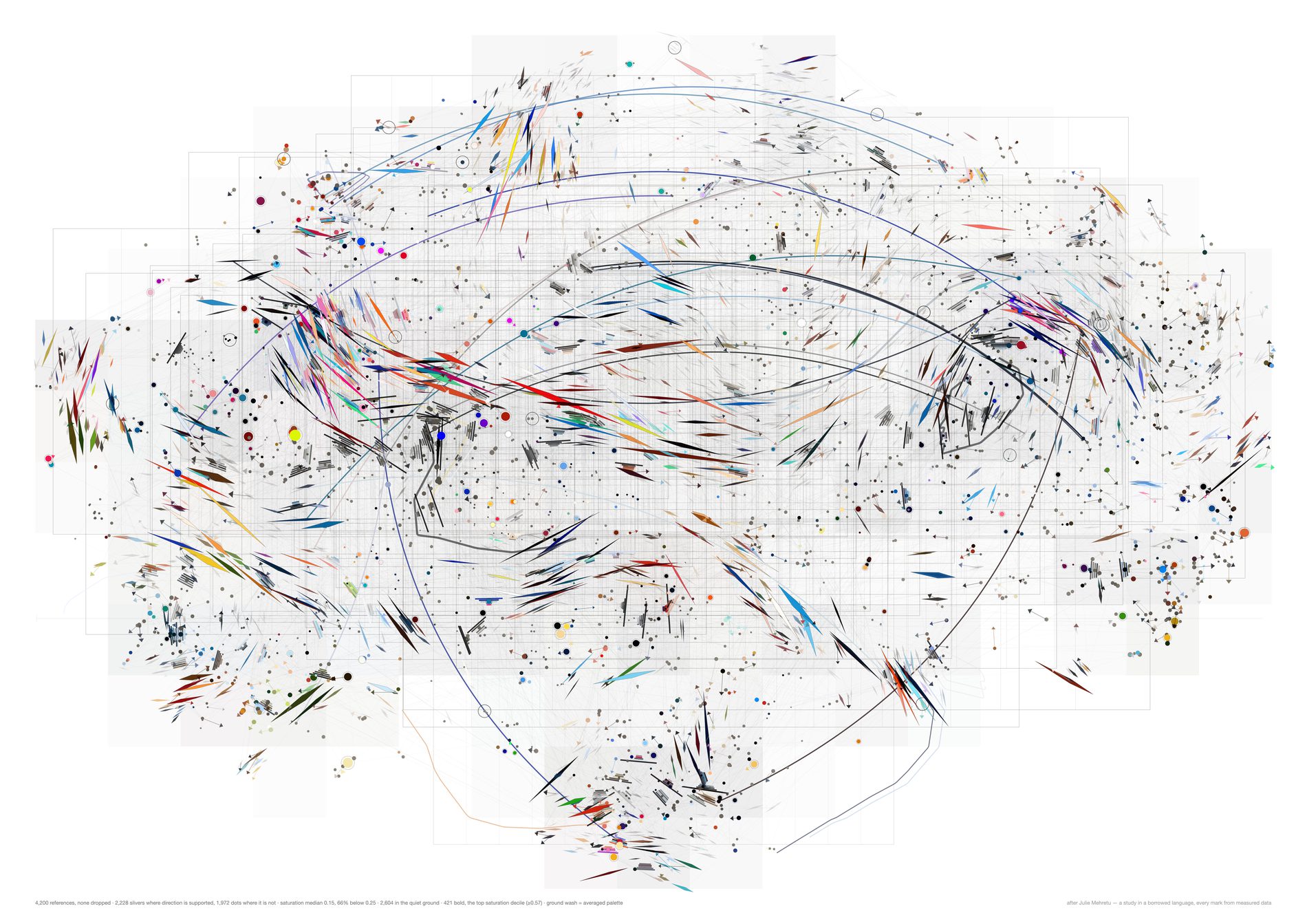
The ground is everything below the colour gate — graphite, at reduced opacity and 0.78 of the previous size, closer to the paper and no longer competing. The middle is drawn in its own measured vivid at normal weight. The bold set is a hard top decile at real strength: 1.7× the length, 1.5× the width, full opacity, and a fine ink keyline on the dots so they sit forward off the ground rather than in it.
Nothing is thinned to achieve this. All 4,200 references are still drawn, and the caption prints the saturation distribution on every sheet — median 0.14, 68% below 0.25 — so a reader is told the quiet ground is the majority rather than left to infer that the archive is more colourful than it is.
The bold set here is chosen by pigment, which is a property of the image rather than of the studio. That is the honest reading of the note as written, and it is the better-looking sheet. The next one keeps the drawing identical and swaps the rule, which is where the argument is.
python3 src/viz/mehretu4.py --n 4200 --k 4 --bands 240 --gestures 20 --plan-min 25 --page a2l --dpi 300 --bold-by saturation --ground-by palette --out mehretu4-mixed
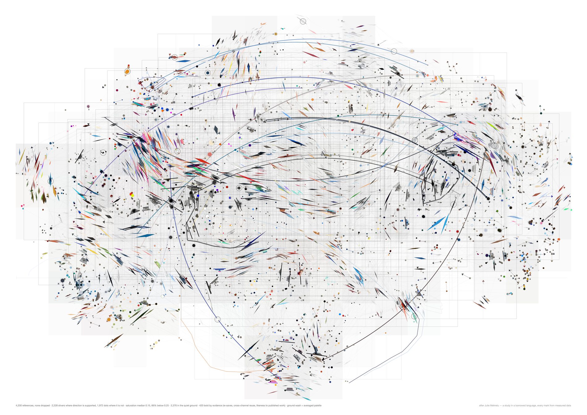
The returns, weight 3.0 — pool.protected(), a pin whose parent pin is also one of FIELD's own, meaning the studio deliberately saved the same picture a second time. 106 are live, and the deduplicator had all 106 in its drop list until src/pool.py put them back. This is the strongest evidence in the archive that somebody came back to something.
The reuse, weight 1.5 per extra channel — a reference filed into more than one channel was carried from one piece of work into another. 1,005 of the pool sit in two or more, 236 in three or more.
The resemblance to what got made, weight 1.0 on the percentile — maximum cosine similarity to any of the 1,086 embedded images of FIELD's own published work. Not proof of influence, but the closest available measurement of “this turned up in the output”. Custody and provenance are deliberately kept out of the score and used for the ground instead, so the two halves of the sheet are not saying the same thing twice.
The measurement cannot settle which bold rule is better. Against a null that permutes the labels across the same positions, the evidence bold set clusters at 30.4% tighter than chance — and the saturation bold set clusters at 31.2%. So the number says both bold sets are spatially structured, which for saturation is unsurprising since CLIP position and colour are correlated, and for evidence is a real finding. It does not say evidence is the better sheet. That argument has to be made on what the marks mean, or not at all.
python3 src/viz/mehretu4.py --n 4200 --k 4 --bands 240 --gestures 20 --plan-min 25 --page a2l --dpi 300 --bold-by evidence --ground-by palette --out mehretu4-evidence
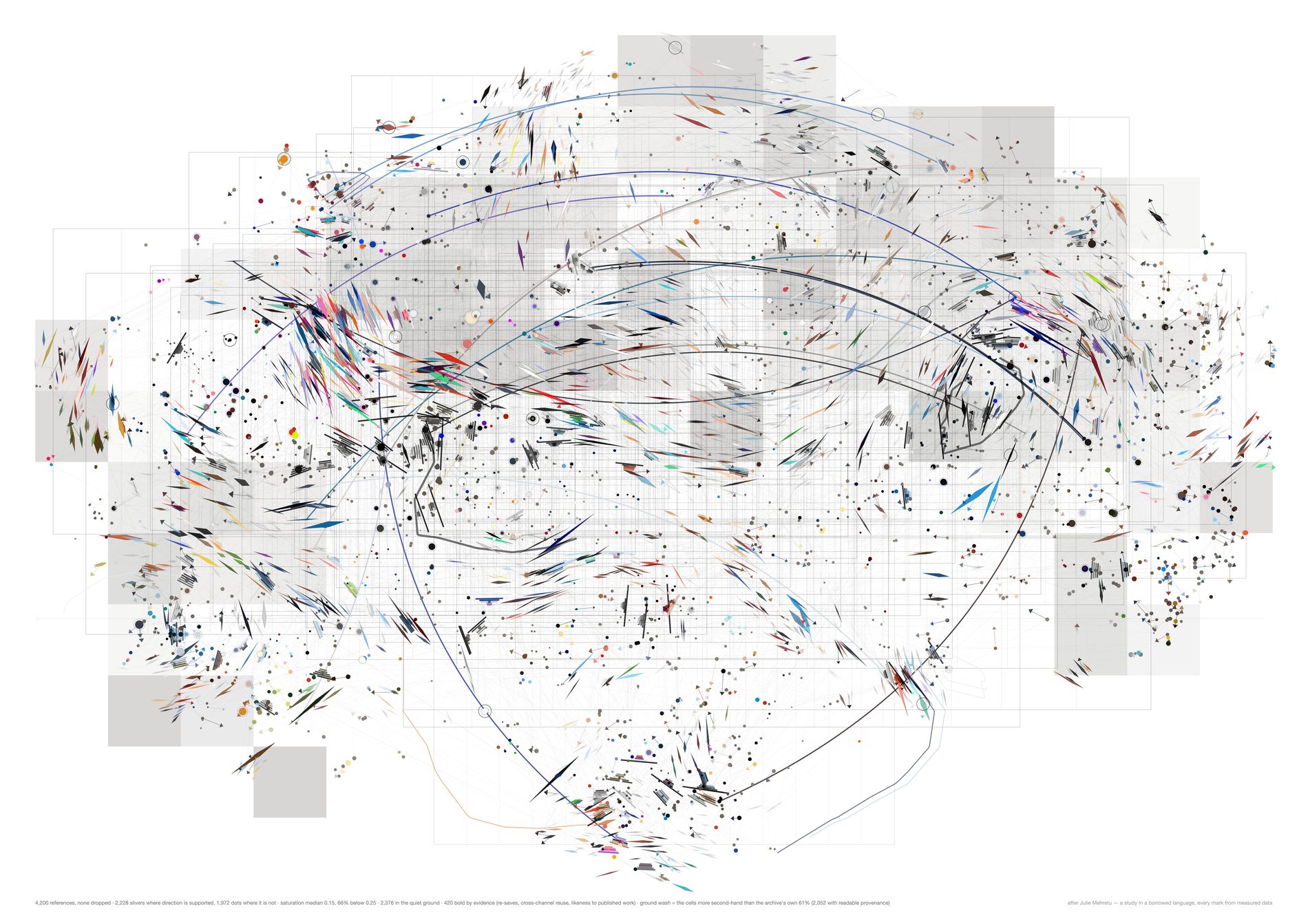
The ground replaces the second and third studies' veils, which averaged five-colour palettes into atmosphere and, by the second study's own control, carried nothing. Here each cell takes ink in proportion to the share of its Pinterest references that were taken from somebody else's board rather than pinned first-hand from a page, and it takes ink only where that share is above the archive's own rate. Across the pool: 6,969 second-hand against 4,163 first-hand, 62.6% of the pins with readable provenance. So the shaded regions are where the studio collected collections and the pale regions are where it found things itself.
A count survives a shuffle by construction rather than by measurement, which is why this layer needs no null. If one thing in this family is meaningful in the sense the note asked for, it is this — and the honest way to say so is that it stopped being a Mehretu move and became a bar chart with the bars laid over a map. Cells with too few readable pins are left as paper rather than guessed at.
Everything else on the page is still a study in a borrowed language with real numbers underneath it. The composition is the t-SNE layout doing the work, as it has been since the first sheet, and the currents still reach about 6% of the page and no further.
python3 src/viz/mehretu4.py --n 4200 --k 4 --bands 240 --gestures 20 --plan-min 25 --page a2l --dpi 300 --bold-by evidence --ground-by secondhand --out mehretu4-secondhand
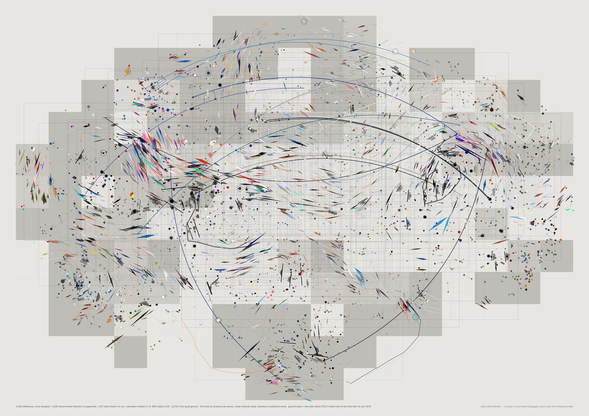
Same construction as the second-hand ground, over a different count: whether a reference has a blob_url, meaning the studio holds the file rather than a link to somebody else's server. 3,158 of 21,491, 19.1%. The biography sheet measured what the other 81% is worth — two in five of what was pinned in 2012 no longer answers.
A wash needs more gain on the house stock than on white, which is the same lesson the third study learned moving the other way: opacity does not survive a change of ground, and the fix is a gain rather than a redraw.
python3 src/viz/mehretu4.py --n 4200 --k 4 --bands 240 --gestures 20 --plan-min 25 --page a2l --dpi 300 --bold-by evidence --ground-by custody --paper "var(--panel)" --veil-gain 1.15 --out mehretu4-custody
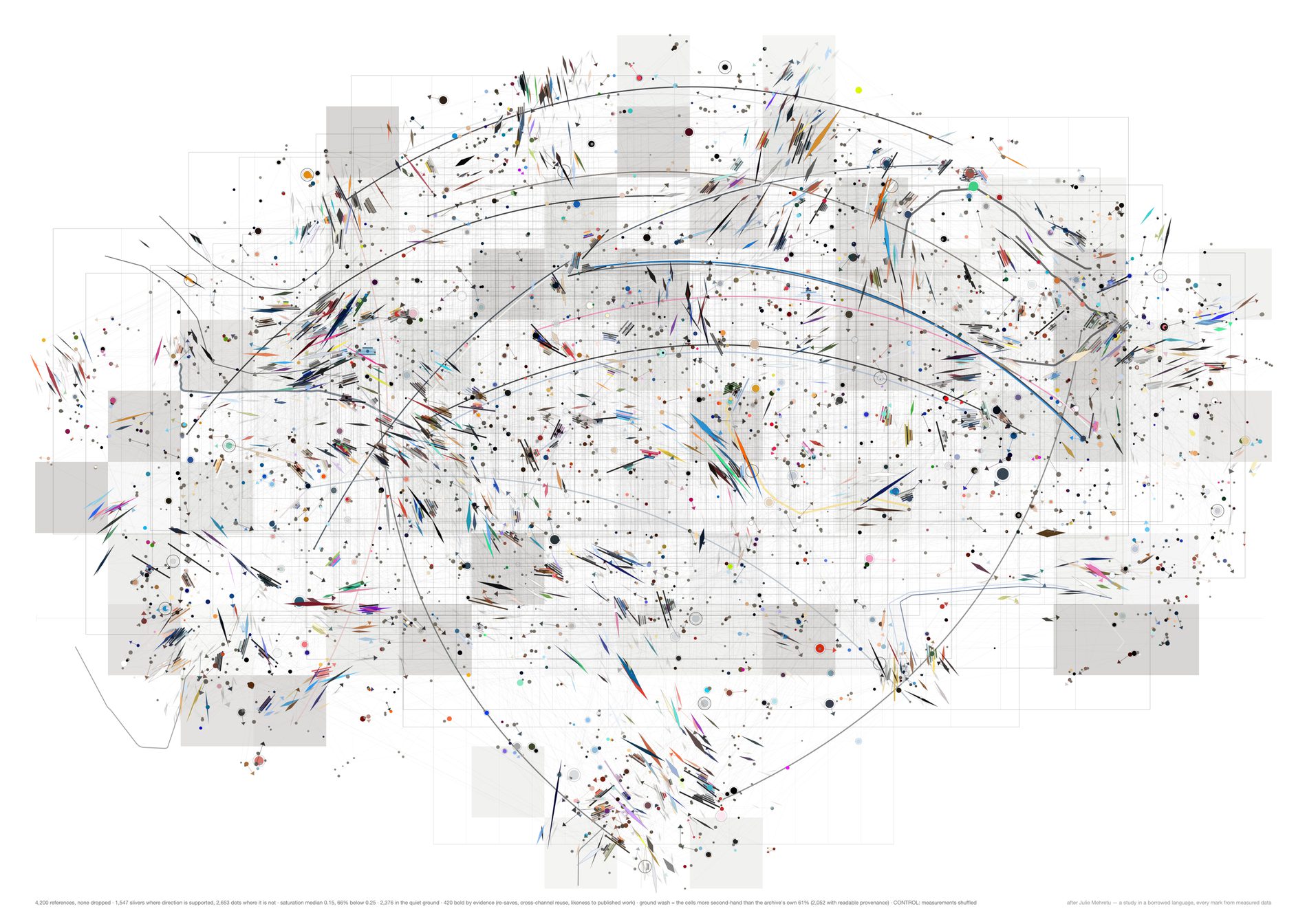
At a fixed support threshold of 0.85, the real sheet earns a direction for 66.5% of its references and the shuffled one for 51.5% — a 15-point difference at n=9,000, and 54.8% against 37.1% at the 4,200 these variants are drawn at.
It holds across the threshold too: +12.6 points at 0.80 and +19.5 at 0.90, so it is a property of the field rather than of one lucky cut.
Why that is a gain over the third study rather than a restatement of it. That sheet's best claim was a 3.1× ratio on a directional correlation — true, checkable, and something no viewer would notice unprompted. This converts the same underlying fact into the vocabulary of the drawing: the sheet stops asserting a direction where its own statistics do not support one, and the share of the page where it declines to is itself the measurement. Nothing was added; something was withdrawn, and the withdrawal is what separates.
The rest of the table did not move, and that is stated rather than buried. At n=9,000 statistics A through F reproduce the third study's published numbers to four significant figures, which is the check that this is the same metric and not a new one wearing the old name. Reducing the grey moved none of them. Pushing 2,358 of 4,200 references into a quiet ground is a decision about looking, not a gain in evidence, and colour was never legible as information on any sheet in this family.
python3 src/viz/mehretu4.py --n 4200 --k 4 --bands 240 --gestures 20 --plan-min 25 --page a2l --bold-by evidence --ground-by secondhand --control shuffle --dpi 130
# python3 src/viz/mehretu4.py --n 9000 --report   # like-for-like with the second and third studies
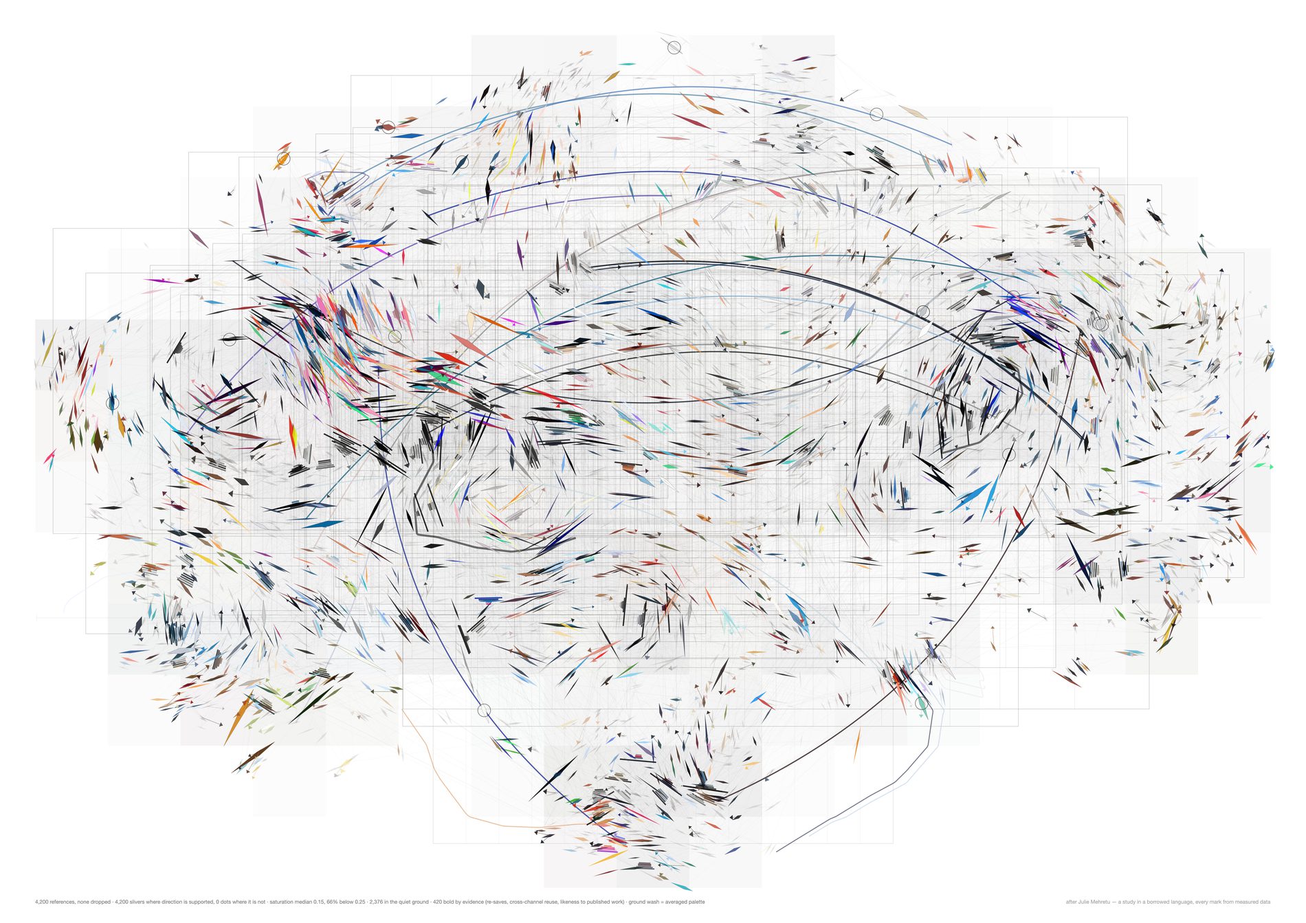
--support 0This is not a study. It is the instrument with one knob at its stop, printed so the vocabulary split can be checked rather than trusted. Every mark asserts a direction, including the half of them whose neighbourhood does not agree on one, which is exactly what the third study did.
python3 src/viz/mehretu4.py --n 4200 --k 4 --bands 240 --gestures 20 --plan-min 25 --page a2l --dpi 300 --support 0 --out mehretu4-vocab-0
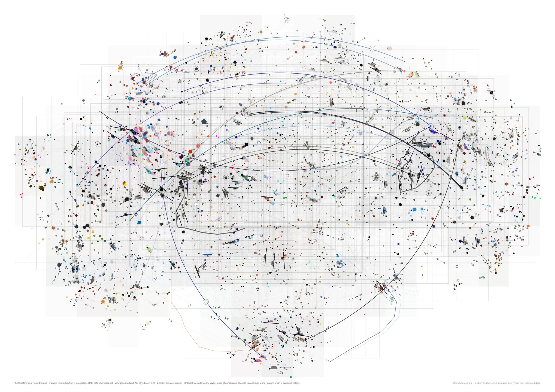
--support 1.1Every mark a dot, none claiming a direction. The first study's vocabulary as a limiting case, against every mark a sliver at the other end.
python3 src/viz/mehretu4.py --n 4200 --k 4 --bands 240 --gestures 20 --plan-min 25 --page a2l --dpi 300 --support 1.1 --out mehretu4-vocab-1.1
Direction 01. Does a new reference still open ground?
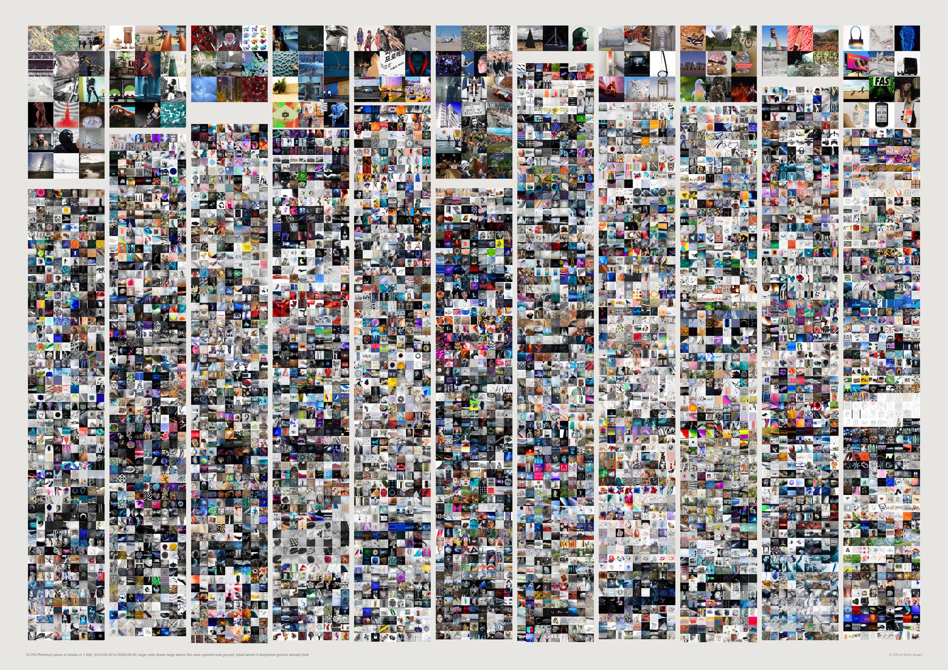
The frontier has not closed. The most recent 238 saves open new ground at 26.9%, against 9.7% for the same references shuffled into a random order. Read the two plates together or not at all: over the whole run they are indistinguishable (16.6% against 16.7%, mean nearest-earlier 0.8398 against 0.8389), and the entire difference is in the shape.
pool(), aesthetic filter on. This asks what the studio looks at, so a link card pasted into a thread cannot be allowed to count as a save with an eye behind it — it is maximally unlike the photographs around it and would read as frontier every time. 11,779 dated Pinterest saves become 11,238.
Novelty yield falls by arithmetic alone: the thousandth save has 999 things to resemble, the eleven-thousandth has 10,999. Any “distance to nearest earlier neighbour” curve slopes upward in any growing collection. The shuffled plate is what pure accumulation looks like.
First block: 26.9% real against 33.7% shuffled. Eleventh: 13.4% against 12.0%. Last: 26.9% against 9.7%. Inferred: real collecting arrives in bursts, so the early years produce fewer frontiers than a shuffle; Pinterest capture then collapsed after 2021 and what remained was sparse and various.
A frontier save here is unlike the archive. That is a statement about the collection, not about the picture. Nothing on this sheet is ranked by quality. Moving --frontier from 0.78 changes every percentage; the gap between the two plates holds its direction across the range.
What would make this wrong. The pool is Pinterest only, because it is the one surface whose dates carry a real chronology — and its capture fell from 2,742 saves in 2020 to 207 in 2026, so the right-hand columns are drawn from a thinning surface. If FIELD's newest looking moved to Basecamp and Figma, and that looking is more familiar than what it pins, this sheet cannot see it. The claim is about the Pinterest habit, not about the studio's whole eye. The last column is 238 saves, not 1,000.
python3 src/viz/d01_frontier.py --dpi 200
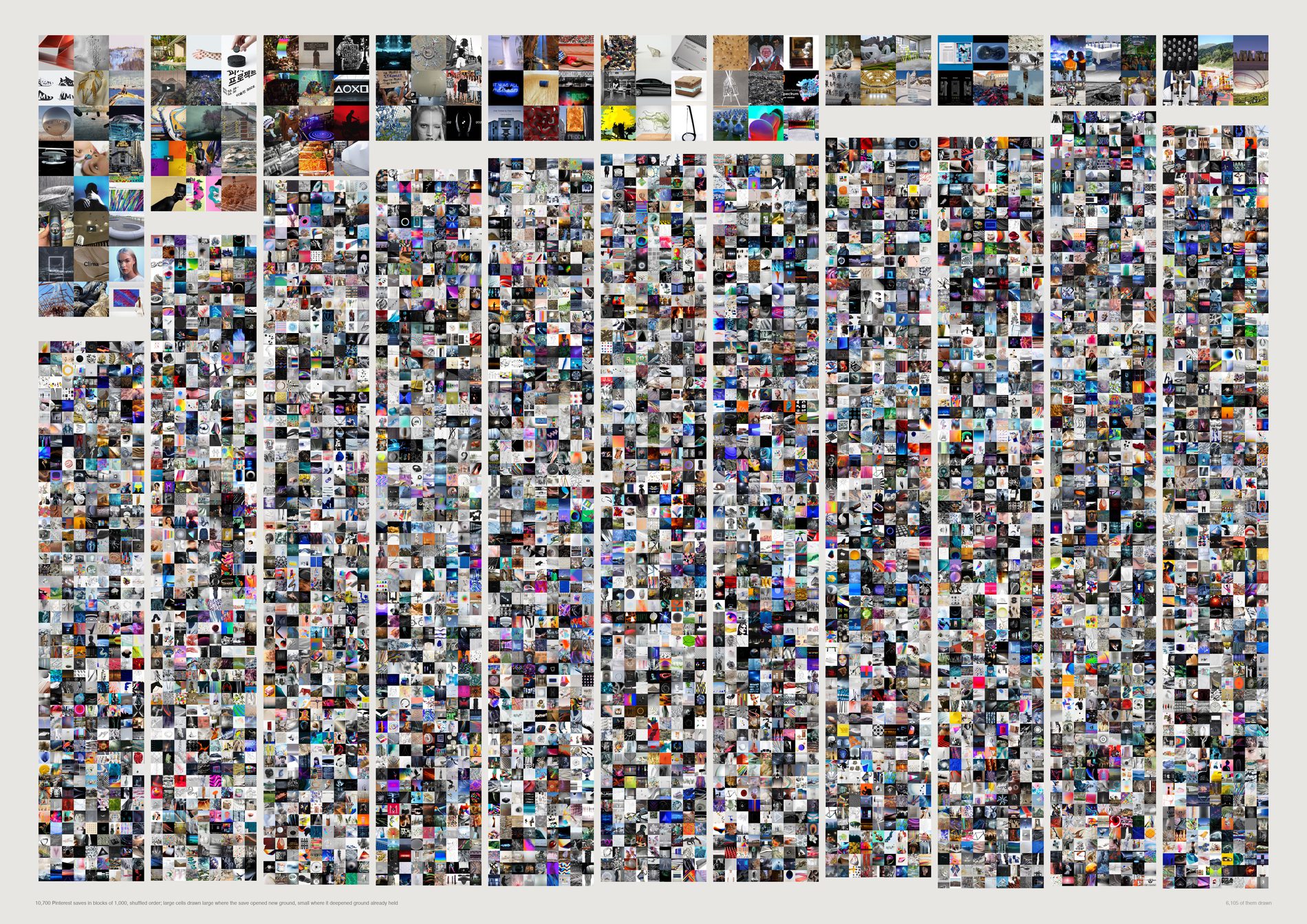
This is what a closing frontier actually looks like, and it is what you get for free from a collection simply getting bigger. The shuffled rate falls by two thirds from beginning to end, monotonically. The real archive's does not fall at all. Publishing the finding without this plate beside it would be publishing arithmetic as insight.
The two plates are the same instrument at the same scale, so the comparison is made by eye rather than taken on trust. A reader who does not believe the percentages can still see that one coarse band thins and the other does not.
The same references, the same 120 k-means regions, the same 0.78 threshold, the same seed. Only the order changes. Territory coverage saturates in both: 120 of 120 regions are occupied by save 10,000 either way.
What would make this wrong. One shuffle is one draw. The seed is fixed at 0 so the plate is reproducible, but a single permutation is not a distribution — the block-level percentages here carry sampling noise that the printed figures do not show. The direction of the effect is stable; the individual cells are not.
python3 src/viz/d01_frontier.py --null --dpi 200
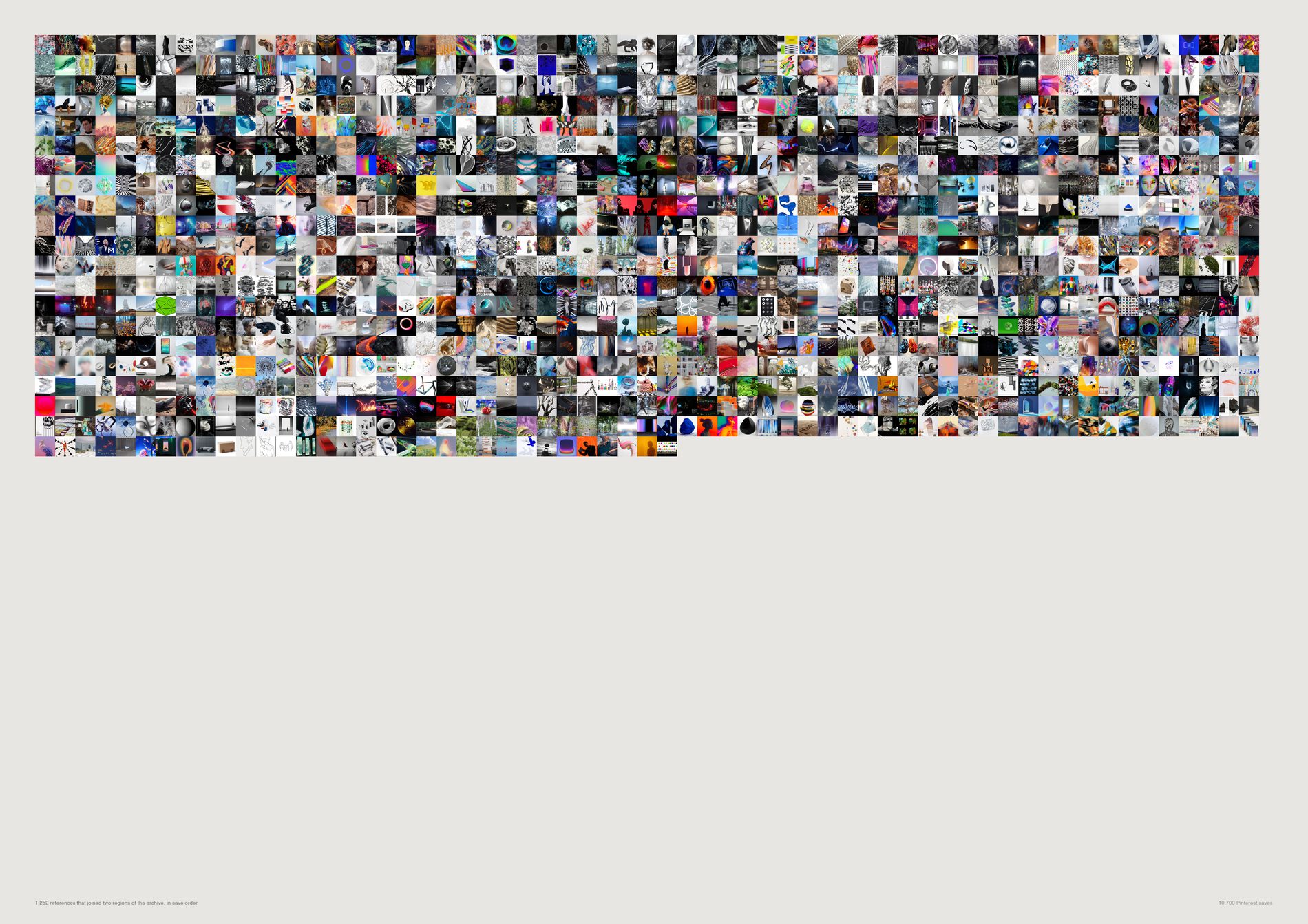
Nothing about the real sequence produces more connections than chance. 1,352 bridges as collected against 1,340 shuffled, and both decline the same way for the same finite reason: there are only so many pairs of regions to join, and the early saves join them.
The hypothesis that the studio's actual order builds bridges was tested and it is a null.
Which pairs got joined is interesting. How many is not. The sheet is kept as a picture of the joins and the count is retracted in the caption rather than quietly dropped from the file.
A bridge is defined against a k-means partition of a continuum, so it is a claim about an analytical boundary rather than about anything the archive declares. Frontier and infill survive the region count moving; the bridge set does not.
What would make this wrong. Beyond the region-boundary problem: the decline is confounded with the block size at the right-hand edge, where the last block holds 238 saves rather than 1,000 (13 bridges real, 22 shuffled — too few to read). Compare the eleventh block instead, 76 against 63, which is the same story at full width.
python3 src/viz/d01_frontier.py --mode bridges
Direction 02. Paths of attention
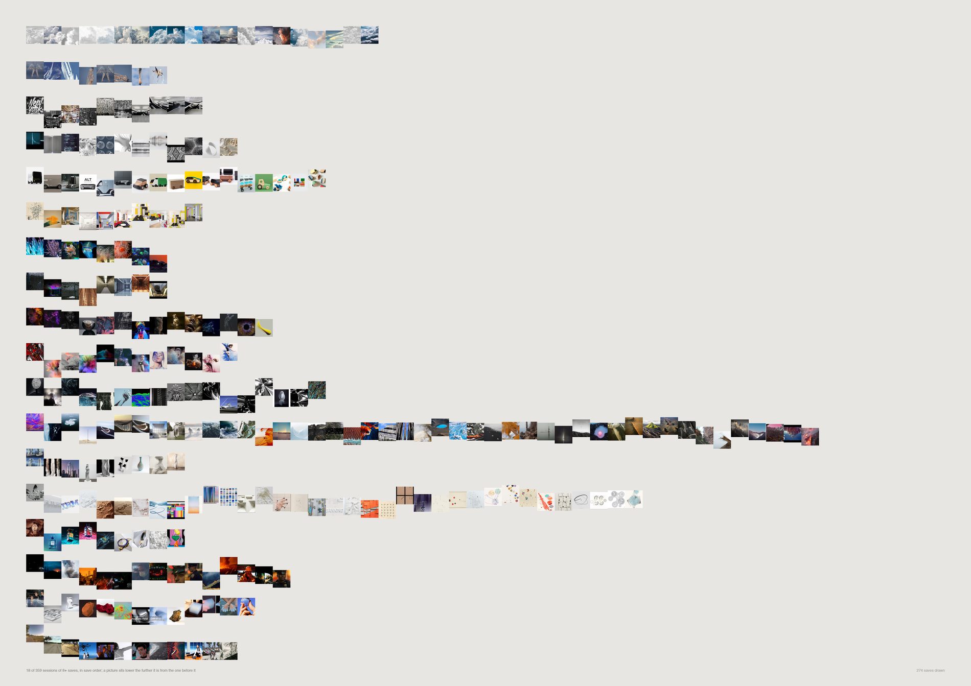
The order of saving carries real information, and its grain is minutes. Consecutive saves sit at 0.7024; the same sessions with their own order shuffled sit at 0.6682; random pairs from anywhere in the archive at 0.5971.
356 of 385 sessions beat their own shuffle, sign test p = 5.0e−73.
pool(), aesthetic filter on, via src/d01_spine.py. A session is a claim about looking, and a run of pasted link cards is a burst of activity with no looking in it. 11,238 saves.
A session is about something (0.668 against 0.597 for the archive at large) and that is most of the coherence. The order within a session adds +0.034 on top, and that is the part only a walk can produce.
Under 10 seconds, 0.7590 (n=513). 10–60 seconds, 0.7314 (n=2,178). One to five minutes, 0.6837 (n=1,854). Five to thirty, 0.6544 (n=1,081). Over thirty, 0.6428 (n=222). Dropping every sub-10-second pair leaves 0.7314, still well clear of the 0.6682 shuffle, so this is not an artefact of batch saving.
Ordered by mean step size and described, never scored: 125 circling, 97 tunnelling, 97 scanning, 46 drifting, 20 mixed. Distance is a change of subject, not a better idea.
What would make this wrong. One account is not provably one pair of eyes — Substrate does not record who pinned, so two people working in the same hour are drawn as one walk. The 60-minute gap is a choice with nothing in the data to anchor it: 30, 60 and 120 minutes give different session counts over the same saves, and the median gap between consecutive saves is 67 seconds with no second mode to cut at. And vertical position is a step size, not a direction: a session oscillating between two territories and one walking steadily away both draw as a jagged line.
python3 src/viz/d02_walk.py --dpi 200
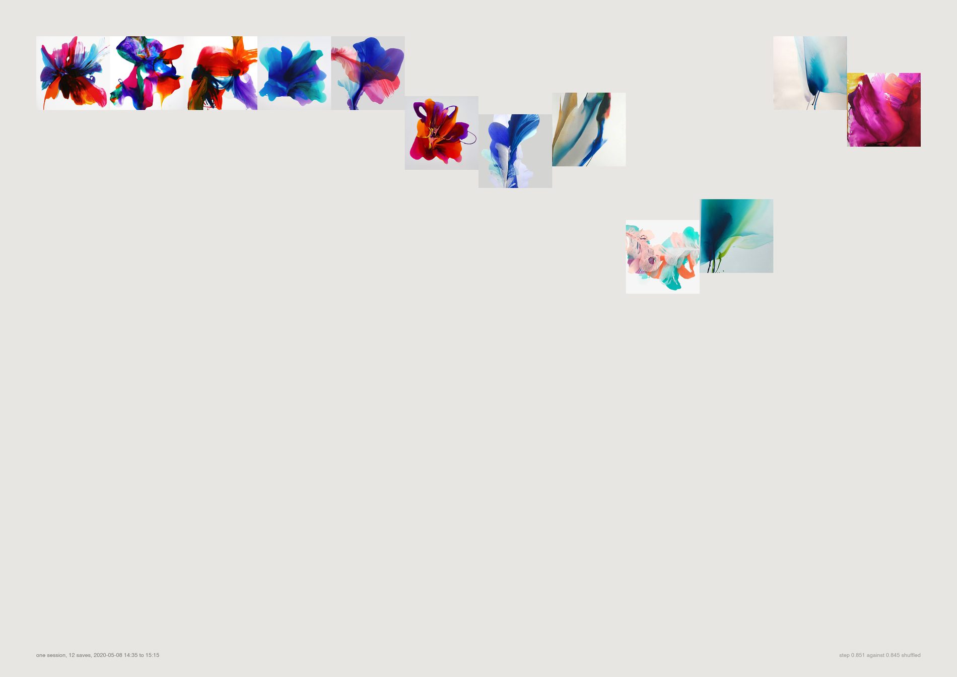
The aggregate sheet carries the effect and hides the thing itself. At this size you can see what a step of 0.70 actually looks like between two pictures, which is the only way to judge whether the measurement means anything.
What would make this wrong. It is one session, chosen by index rather than by argument, and it carries no statistical weight at all. Nothing on this page should be generalised; the numbers live on the full sheet.
python3 src/viz/d02_walk.py --one 3 --page a3l
Direction 03. Does project research converge?
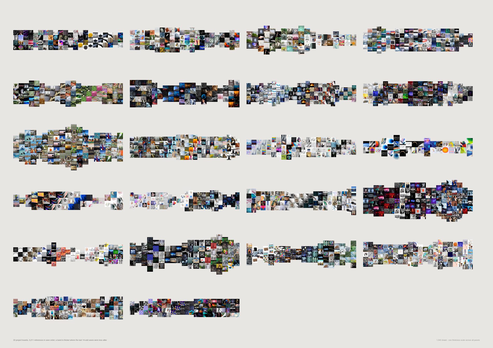
Project research does not systematically converge. Against 300 shuffles of each board's own saves, two boards narrow significantly where about 0.6 would be expected by chance, none widen, and the mean correlation of spread against position is −0.039 — a tilt nobody could act on.
Diverge-then-converge is a story the archive declines to tell.
pool(), aesthetic filter on, via src/d01_spine.py. The board count fell from 26 to 23 when the filter was applied: three boards no longer clear 100 usable references, which is itself worth knowing about how much of some project research was screenshots.
242 Swisscom Energy Air — Dance! (r = −0.856, p = 0.007) and PG2 (r = −0.657, p = 0.033). Real individual shapes, not evidence of a studio process. A third, P108 UAE Expo Pavillion, lands at p = 0.050 and is not counted.
How often does a board reach into a region it has not used yet, first third against last? That rate falls by +0.292 across a project — and falls by +0.366 in the shuffled order. Any accumulating set runs out of unused regions whether or not anyone was converging, and the arithmetic accounts for more than the whole observed decline.
Some of these projects needed late disruption and some needed sustained focus. No panel is scored, and --sort number puts them in plain project order for anyone who finds the shape-ordering suggestive.
What would make this wrong. A Pinterest board is not a project's research — it is the part that got pinned, and a band that thins may mean the looking moved somewhere Substrate cannot see. Save order is not necessarily thinking order: boards get reorganised and old pins get added to new boards, which trimming to the densest 80% of each date range reduces but cannot remove. And 23 boards is a small n; a larger corpus could turn this null into a weak finding in the narrowing direction. It could not turn it into the textbook curve.
python3 src/viz/d03_breathes.py --dpi 200
Direction 05. The lifespan of a visual idea
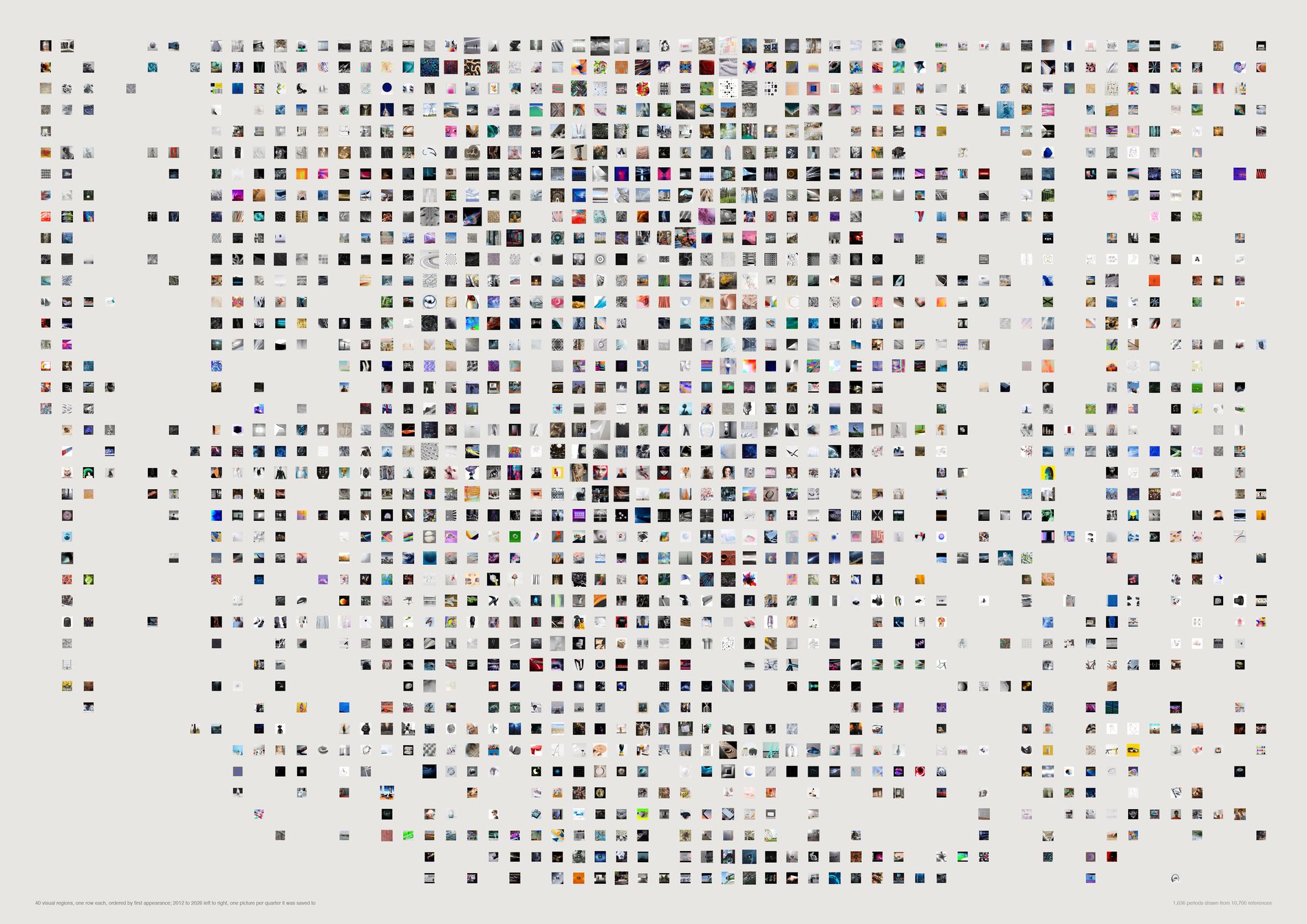
FIELD does not abandon visual ideas, and when it comes back it comes back to the same pictures. Not one of the 40 regions flashes and dies. 25 go quiet for a year or more and return — and the centroid of what was saved after a dormancy matches the centroid before it at a median cosine of 0.912 (range 0.705 to 0.980).
The poetic reading — a dormant idea returning transformed — is not what this measures. The returns are not transformed.
pool(), aesthetic filter on, via src/d01_spine.py. Persistence is a claim about a continuing interest; a region kept alive by recurring screenshots is not one. 11,779 dated saves become 11,238.
This sits alongside four already established in the repo — no colour drift, no complexity drift, stable CLIP year-centroids, no subject or mood trend — and says the same thing from a fifth direction. The eye did not change, and it did not drop anything either.
At the default floor of 1, a region with a single save in a quarter is drawn as active. That is the maximally generous setting about persistence, which is the conservative direction for a sheet arguing that things stop. --floor raises the bar.
What would make this wrong. The clock is Pinterest's, and Pinterest capture fell from 2,742 references in 2020 to 207 in 2026 — so the right-hand edge of every row thins for a reason that has nothing to do with the idea. A region going quiet after 2021 may be a region going quiet, or the studio's collecting moving to Basecamp and Figma where this sheet cannot follow it, and nothing here separates those. Regions are k-means cuts through a continuum; --k moves every lifespan on the sheet. Nothing here is ranked: a flash is not a failure.
python3 src/viz/d05_halflife.py --dpi 200
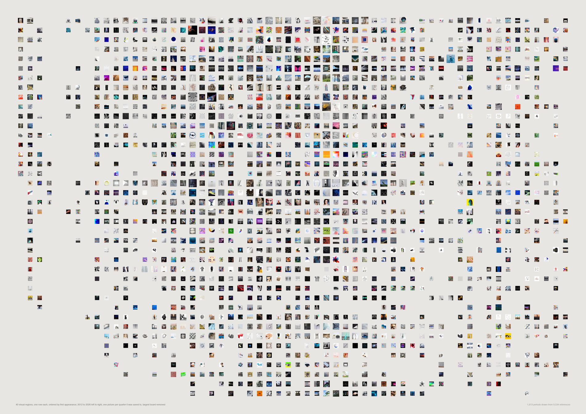
The persistence survives the surgery. A region lighting up in 2018 and again in 2023 looks like a recurring interest and could just as easily be two unrelated jobs that needed similar pictures. Delete every region's dominant board and nothing moves: 31 still continuous, still no flashes, one more region returning, and the before-against-after cosine falls from 0.912 to 0.907. Only one region in forty is half-supplied by a single board in the first place (X Activist Aesthetics, 63%).
It is the honest version of the sheet, and any claim made from the first plate has to survive it. In this archive it does. A row that emptied here was one project all along and the recurrence was never a cycle.
In this plate the terminal's largest board column divides the removed board's original count by the reduced total, so it prints impossible shares (X Activist Aesthetics reads “169%”). Nothing on the sheet uses that column and no number in this caption comes from it — the guardrail figure quoted above is from the full run. It is recorded here rather than fixed silently.
What would make this wrong. Removing the largest board removes about 11% of the references and does not remove the second-largest, so a region carried by two big jobs still survives this cut. It is a test against single-board dominance, not against project-driven persistence in general.
python3 src/viz/d05_halflife.py --without-top --dpi 200
Direction 04. Research personalities
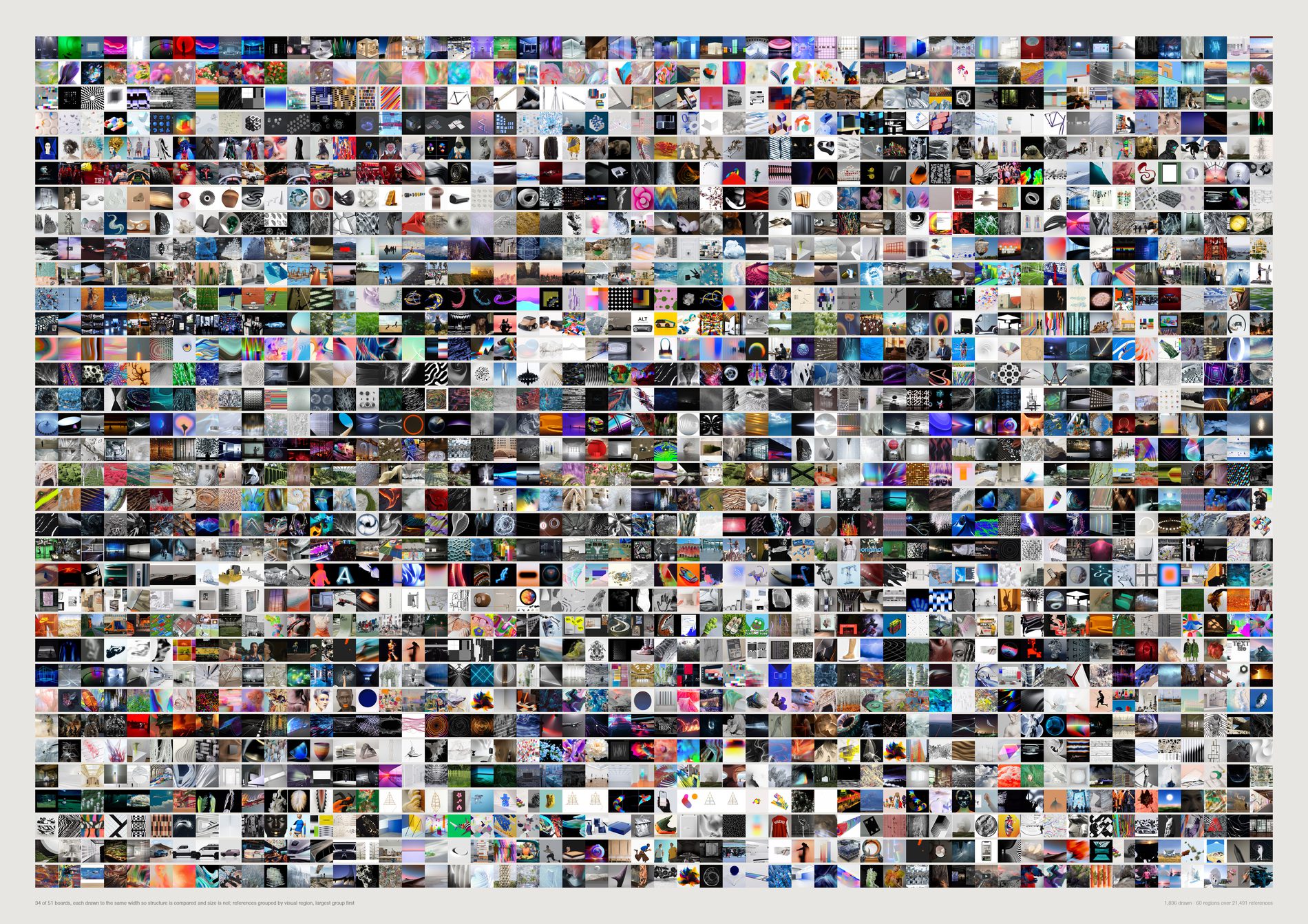
Research structure varies far more than volume does. Two boards of almost identical size sit at opposite ends of the range: 242 Swisscom Energy Air — Dance! at 105 references occupies 24 regions with 46% of itself in one, and Culture at 113 references occupies 41 with no region above 11%.
pool(), aesthetic filter on, via src/d01_spine.py. A board's breadth is a claim about the eye, and a board padded with link cards would read as broad for a reason that has nothing to do with looking. 26,214 references become 21,491; 63 qualifying boards become 51.
Entropy rises with sample size for pure arithmetic reasons, so every board is subsampled to the same 100 references before it is measured. Raw, entropy against board size is r = +0.444; controlled, r = +0.177. The control removes about 60% of the relationship and does not remove all of it. Read the ordering as “structure, partly confounded with scale”.
One k-means over all 21,491 references, not one per board. A board's breadth has to be measured against the archive's territory, not against a partition drawn around the board itself.
Exploratory 13, fragmented 7, obsessive 5, tightly resolved 3, panoramic 2, bifurcated 2, concentrated 1. The names print to the terminal and appear nowhere on the sheet; rows are ordered by a measurement, and nothing computes a score. Obsessive is not worse than panoramic.
What would make this wrong. Regions are cut, not found — --k changes every number here, and while the ordering of boards is stable from k = 40 to 120 the individual region counts are not. A board is not a project but the pinned part of one, and several channels under Projects are places rather than jobs (Beirut, Hong Kong, Munich, Seoul), which is a known pollution in this repo's channel data. And repetition is measured on what survived deduplication: the genuinely duplicated saves, which would be the strongest evidence of obsession, are the ones the pool throws away first.
python3 src/viz/d04_personality.py --dpi 200
Direction 08. The pictures the categories cannot hold
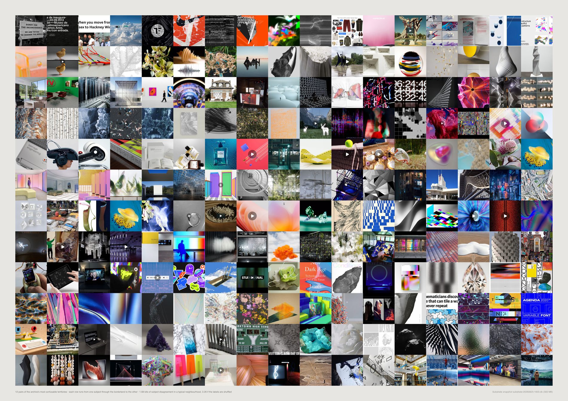
“Ambiguous” is four different sets, and one of them shares nothing with the others. Of the top 48 by each definition: neighbourhood entropy and self-disagreement share 37, entropy and cross-model disagreement share 27, self and cross-model share 33 — and “sits on a boundary between two clusters” shares 0 of 48 with all three. A reference near a seam in the partition is not the same object as a reference whose visual company cannot agree what it is.
pool(aesthetic_filter=False). This is the one sheet in the set that is about the method as much as the pictures: its stated job is to separate productive ambiguity from analytical failure. Filtering the failure cases out upstream would let it claim a cleanliness it had not earned, and the guardrail would stop being checkable. The filter off, the population goes up — 19,209 to 19,315 — because the 106 deliberate re-saves come back and nothing is removed. 18,113 of those carry a subject label and both models.
The vision model returns unclear on 40 subjects, 0.22% (and 340 mediums, 1.88%). That is a measure of how reluctant a language model is to refuse a multiple-choice question, not a measure of ambiguity. It is reported and set aside.
The closest subject centres: typography | graphic 0.980, texture | abstract 0.977, object | sculpture 0.974, interior | installation 0.973. The first pair only exists because the aesthetic filter is off here, which is the decision above doing visible work.
A reference's own label differs from its neighbourhood's majority 44.0% of the time, and the two CLIP models' neighbourhoods vote for different subjects 27.4% of the time. Nothing is labelled on the sheet: either the two ends look like two different things and the middle looks like neither, or the row has nothing to say.
What would make this wrong. Neighbourhood entropy is bounded by the label set — with 27 subjects of wildly uneven frequency, a reference sitting among the three biggest scores higher than one among the three smallest for no reason to do with the picture. That is why the shuffled control (3.32 bits, against a 4.32 ceiling) is printed beside the real 1.75. And a borderland between two model-assigned labels is not a borderland in the world: these are the seams of one taxonomy chosen by one model, and a different list of subjects would put them elsewhere.
python3 src/viz/d08_ambiguous.py --dpi 300
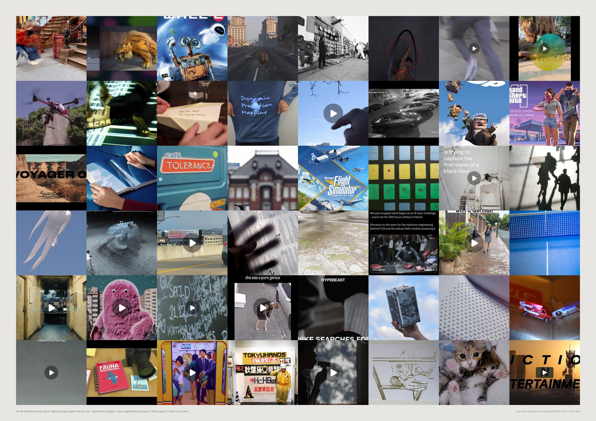
Null, and in the opposite direction to the one predicted. The claim was that references resisting a settled identity get reinterpreted across more briefs. Correlation between neighbourhood entropy and channel count: r = −0.050.
The most ambiguous tenth sits in 1.05 channels, the least ambiguous tenth in 1.12. Filed in more than one channel at all: 3.7% of the most ambiguous tenth against 8.3% of the least, 5.8% overall.
And the test was underpowered before it started. The mean reference sits in 1.08 channels. There is almost no reuse in Substrate to correlate anything with, so no version of this test could have produced strong support in either direction. Both halves of that have to be said: the sign is against the claim, and the instrument was too blunt to have settled it.
It is consistent across three different cuts of the same data — the correlation, the mean channel count by decile, and the share filed more than once. A weak test that points the same way three times is not evidence for the claim.
The deeper problem, and it is not fixable from inside this archive. A reference that appeared in one board and shaped a whole job looks identical here to one nobody opened twice. What can honestly be said is narrow: this archive holds no evidence for the claim, and a little against it.
What would make this wrong. Channel membership is the only reuse signal Substrate records, and it is a filing act rather than a use. If FIELD reuses references by looking at them again rather than by re-filing them, this test is measuring the wrong thing entirely — and at a base rate of 1.08 channels per reference, that is the more likely reading. The correlation is also computed over references that carry a subject label and both models, which is 18,113 of the 19,315 in the pool.
python3 src/viz/d08_ambiguous.py --plate fog --dpi 300
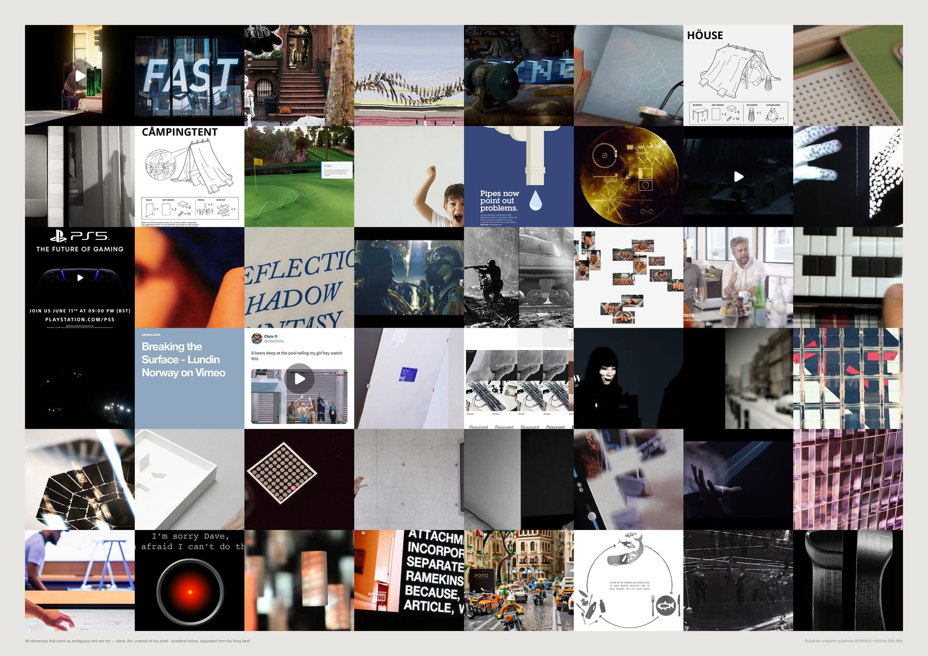
A blank scan is genuinely unlike everything and genuinely unclassifiable, and it is not what direction 08 is about. Without this floor, a quarter of the “most ambiguous” list is bad files. The floor is drawn rather than asserted, so the judgement can be checked by eye instead of trusted.
The brief's instruction was to separate productive ambiguity from analytical failure “where possible”. A filter that removes a quarter of the candidate set is a large intervention, and a sheet that applied it silently would be making an aesthetic judgement while claiming to make a measurement.
Four crude tests stand in for one hard judgement. A deliberately flat, low-contrast photograph is indistinguishable to them from a bad scan, so some real references are on this page. That is the direction the error runs, and it is the conservative one.
What would make this wrong. The four thresholds are chosen, not derived — bottom-decile entropy, near-zero edge density, blown or crushed median brightness, under 200px on the short edge — and moving any of them moves the 23.9%. The floor also cannot see a well-exposed, sharply-focused image that is nonetheless a screenshot of text, which is the case the aesthetic filter would catch and this sheet deliberately leaves off.
python3 src/viz/d08_ambiguous.py --plate thin --dpi 300
Direction 09. The syntax beneath the subject
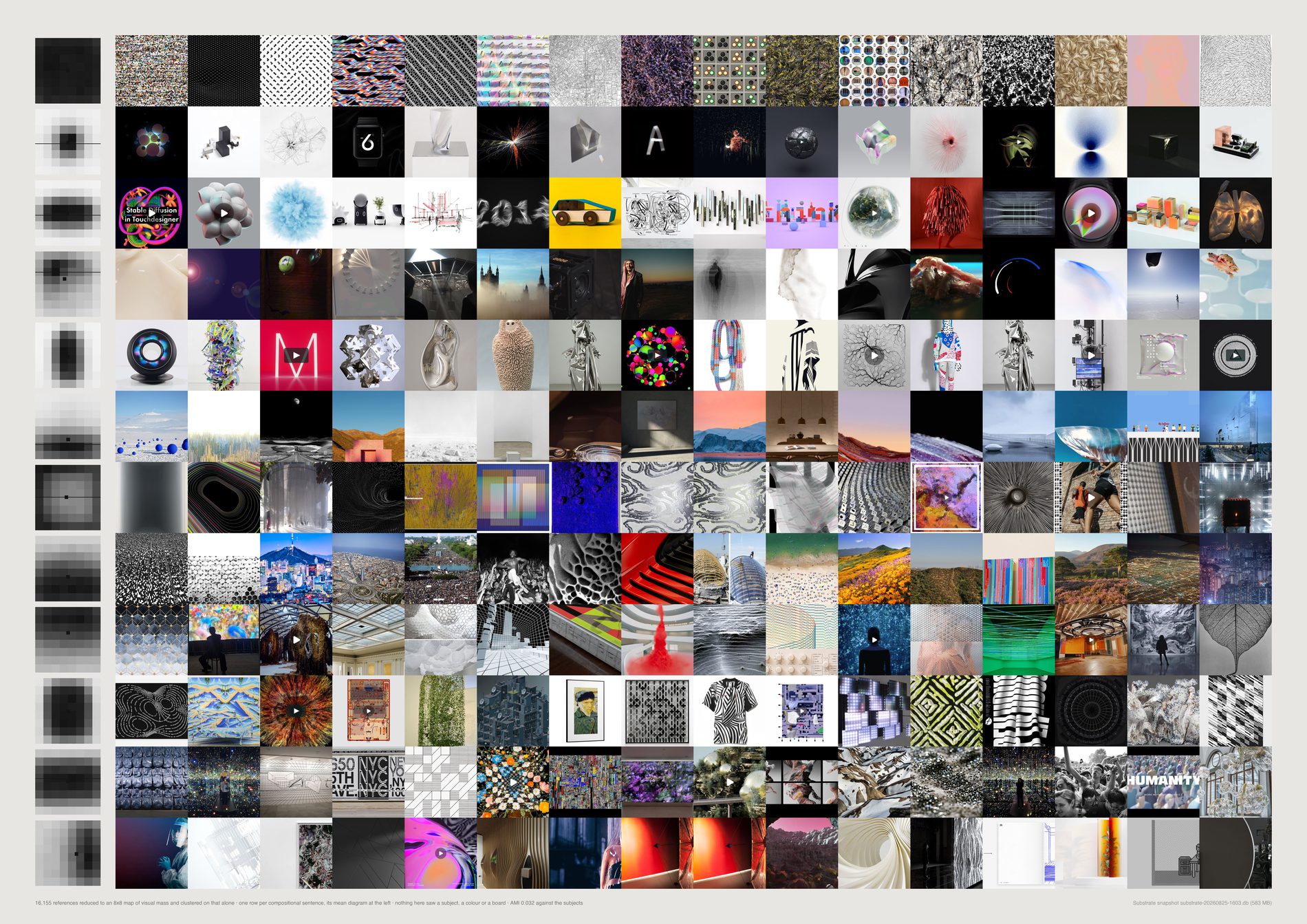
Arrangement is near-orthogonal to content. A low AMI is the good outcome here and the opposite of what it means in clusters.py: at 0.035 against the vision model's subjects and 0.006 against its mediums, the compositional axis is carrying information the subject axis does not.
A photograph of a face and a render of a turbine land in the same group if they are arranged the same way.
pool(), aesthetic filter on. Composition is a claim about how the studio's material is arranged, and a screenshot of a text post has a strong compositional signature — horizontal bands, high emptiness — that would take one of only twelve rows for a non-aesthetic reason. 19,209 references become 17,499.
The 999 published works are distributed across the twelve sentences differently from the 17,499 collected references: chi-square 19.7 against a null median of 9.6, permutation p = 0.037, largest enrichment x1.35. On the unfiltered population this test read chi-square 27.5, p = 0.004, x1.42. The effect is roughly half as strong on the pool and now sits just inside 0.05. It is a lean, not a house style.
The over-used sentence (81 of 999 published against 1,050 collected, x1.35) is characterised as mass_x +1.5 · sym_lr −1.0. mass_x scores 0.002 on the validity table and is flagged do-not-quote; sym_lr scores 0.032. The clustering is on the full 64-cell diagram, so the cluster is real — but the words describing it are not load-bearing, and this caption will not pretend otherwise.
Not subject, colour, client, year or board. If the rows work, twelve unrelated things look like variations of one arrangement. --k varies the count and the AMI prints each time; if the headline moved with k, the finding would be about the parameter.
What would make this wrong. Gradient energy is a poor stand-in for attention: a quiet subject against a busy ground has its measured mass in the ground, so some rows are rows about where the texture is. Eight by eight is a coarse diagram — it cannot tell one object from two touching ones, and anything below a fiftieth of the frame is invisible to it. And the diagram squashes where the sheet crops: d09_compose.py resizes to 128×128 without cropping, so a panorama is measured as if it were square, while the page centre-crops. A very wide reference is where the picture and the row diverge most.
python3 src/viz/d09_grammar.py --dpi 300
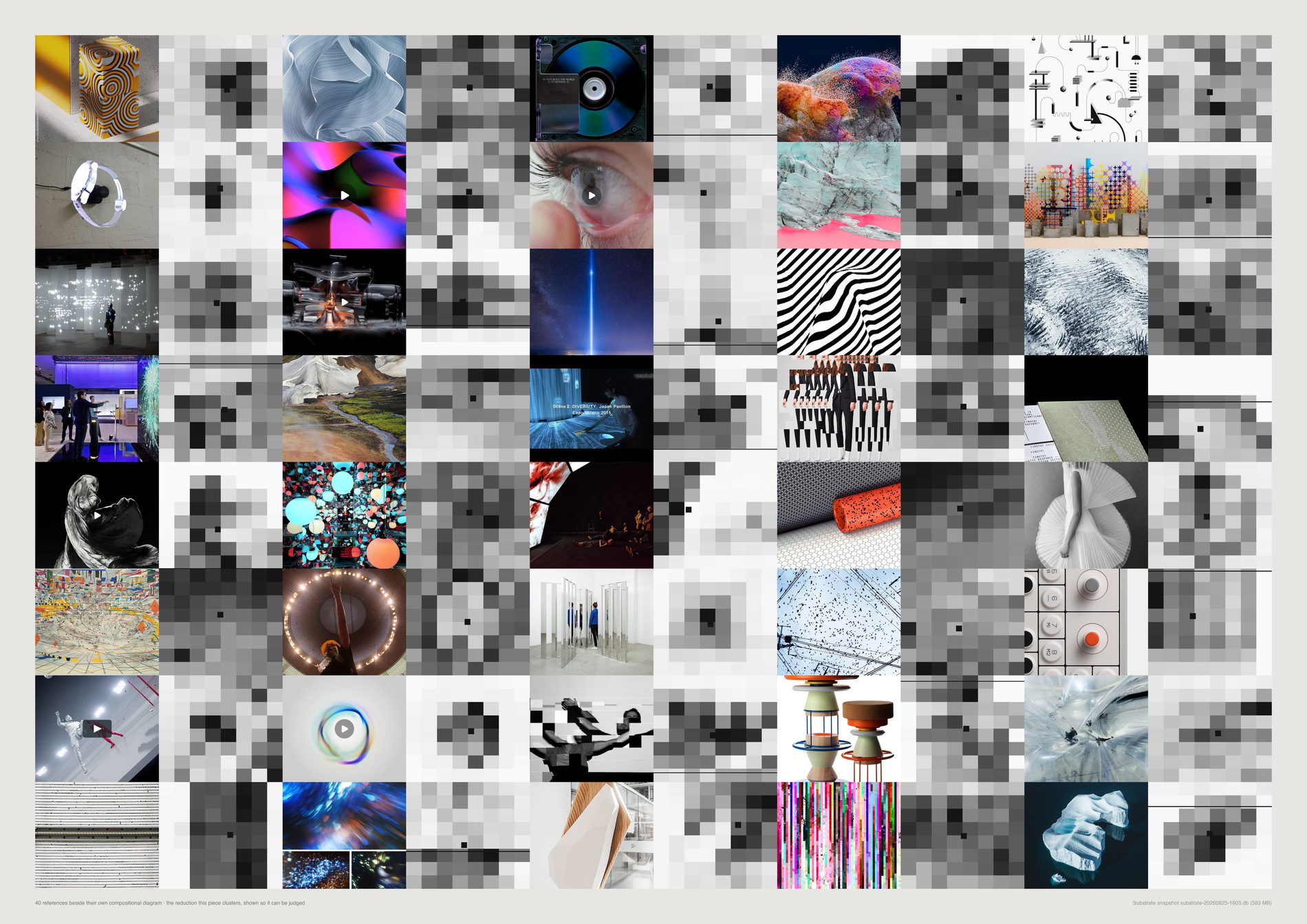
Four of the sixteen compositional measures carry no signal, and the two the brief leaned on hardest are two of them. thirds scores 0.004 — the rule-of-thirds measure separates nothing at all.
mass_x scores 0.002, horizon 0.010, vp_k (the vanishing-point proxy) 0.016. All four are flagged do not quote on every run.
They stay in the file rather than being deleted, because removing a measure after watching it fail, without saying so, is how a method quietly becomes a story.
empty 0.105 (product +0.57 / texture −0.68), blobs 0.098 (texture +1.00 / product −0.42), spread 0.091, border_share 0.091 (both texture-high, sculpture-low), layers 0.051. Texture running to many small blobs filling the border and sculpture to one centred mass are the directions a person would predict, which is the point of the check.
It scores highest on graphic (horizon_k, 0.026), which have hard horizontal bands and no horizon in them. That is not a weak measure; it is a measure of something else wearing the name.
The brief asked for a check against a human-curated sample and there has been no human check. This plate exists so that one can actually be made: images beside their own diagrams at a size where the two can be compared. The validity table is the machine substitute, and it is scored against a different model's labels rather than against the one that produced the clusters.
What would make this wrong. Between-subject variance is a proxy for validity and a crude one: a measure could capture something real that happens not to vary by subject, and would score zero here. It is evidence that a measure is uninformative about content, which is exactly the argument being made about thirds — but it is not proof that thirds measures nothing at all. The table is computed on the 16,124 pool references the vision model labelled, over the 21 subjects with at least 100 of them.
python3 src/viz/d09_grammar.py --verify --dpi 300
Direction 10. Where the archive puts the viewer
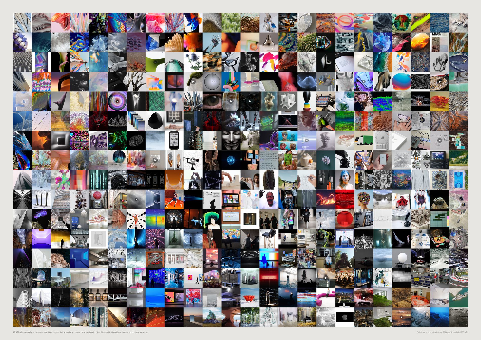
FIELD's archive puts its viewer either inside a field or in front of one object, and hardly ever where a person actually stands. Surrounded 5,428 (31.0%) and confronted 2,260 (12.9%) against eye level: 169 references, 1.0%.
Whatever this studio collects, it is not photographs of the world at head height.
pool(), aesthetic filter on. Where a picture puts you is the plainest possible taste question. It changes one headline honestly: indeterminate falls from 28.3% to 25.5% once the screenshots and pure typography are out, which is the filter removing exactly the material that had no viewpoint because it was not a view. 19,209 references become 17,499.
Camera position is scored by CLIP. Subject is labelled by a different model that never saw these prompts. Eight agreements at x4.2 or better: landscape → distant overview x15.8, architecture → outside x11.2, interior → inside x9.6, landscape → above x6.6, interior → threshold x6.2, person → eye level x6.0, texture → extreme close-up x5.9, architecture → below x5.8. Inferred: agreements that strong between two models sharing no training and no vocabulary are not a coincidence.
Eye level (169), threshold (149), distant overview (109) and looking through (104) all fall under 1%, and the script names them on every run as categories the model can barely tell apart from their neighbours. That includes eye level, which is the number this sheet is built on. The finding is that the category is nearly empty; the exact figure is not a strong measurement.
None is needed. The top of the page is close and the bottom is far, and you can see that it is. Each row is filled by taking a proximity band and spacing it evenly along the elevation ranking, so every cell is a real image.
What would make this wrong. Zero-shot proportions are not calibrated: 31.0% surrounded is a share of this prompt book, not of some absolute truth, and changing the fifteen sentences moves every share. What the sheet supports is the ordering and the relative reading between slices; what it cannot support is “a third of the archive is immersive” as a bare fact. Elevation and proximity are contrasts, not measurements — each is a softmax over two or three of the fifteen categories, so an image with no elevation cue at all still gets a position near the middle, indistinguishable from one genuinely at eye level. And the grid equalises what the archive does not; the counts are printed for that reason.
python3 src/viz/d10_viewer.py --dpi 300
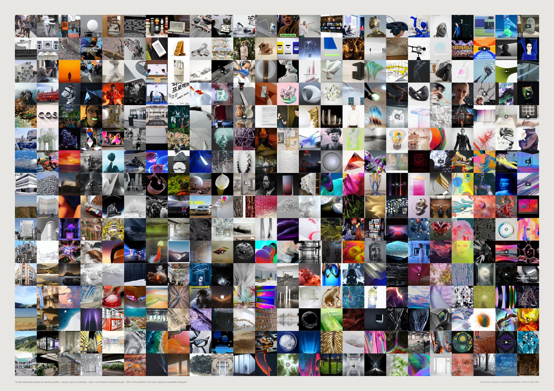
Elevation and proximity are the pair with the strongest external validation, so they carry the finding. Enclosure and aperture are printed because the axes are cheap to swap and the archive reads differently under them — and because a grid that only ever works on one pair of axes is a grid that was fitted to its answer.
What would make this wrong. Nothing here is validated against the second model the way elevation and proximity are, so this page is a study and not evidence. Both axes are softmax contrasts over a handful of the fifteen prompted categories, which means an image with no enclosure cue still lands somewhere.
python3 src/viz/d10_viewer.py --axes enclosure,aperture --dpi 300
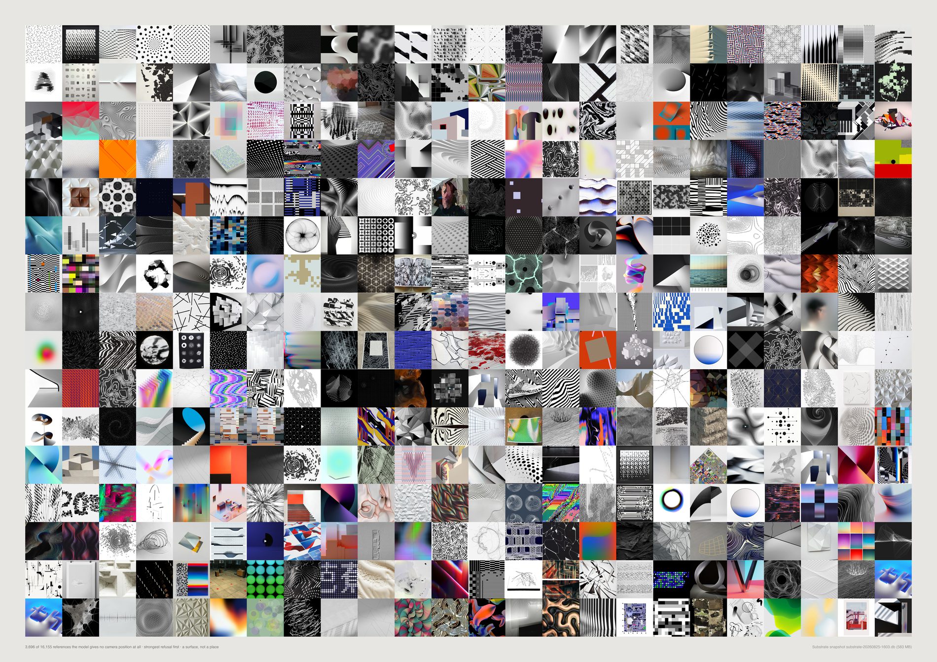
The confidence-margin implementation of “indeterminate” does not work, and it fails in the wrong direction. Tested on 3,154 flat graphics against 3,547 photographs of places: the median top-two margin is 0.0070 for the flat graphics and 0.0057 for the photographs — a working measure would be the other way round.
At every threshold it flags more photographs than graphics: 16% against 20% at margin < 0.002, 31% against 38% at 0.004, 44% against 52% at 0.006, 66% against 71% at 0.010.
The explicit category does work. Given indeterminate as one of the fifteen sentences the model can choose, it picks it for 59% of the flat graphics and 14% of the photographs. Asking the model outright beats inferring from its uncertainty, and the failed version is printed here rather than dropped, because the margin trick is what anyone would try first.
Against the archive's own average: FIELD-OS Branding +46% indeterminate (137 references), Type +43% (149), Graphic +36% (411), 360 IMI +36% (111). The categories that lean in are the ones that should — graphic x2.6, data-visualisation x2.1, abstract x1.5 against a different model's subject labels.
A quarter of the archive is a surface rather than a place, and it is invisible on the main grid by construction. It gets its own sheet rather than a footnote.
On the unfiltered population indeterminate was 28.3%; on the pool it is 25.5%. Some of what had no viewpoint had no viewpoint because it was a screenshot. What is left is material that is genuinely flat by intent.
What would make this wrong. The control uses the vision model's own labels to define “flat graphic” and “photograph of a place”, so it tests agreement between two model outputs rather than against ground truth — a systematic error shared by both would pass it. It is also computed over all 23,036 embedded ids rather than over the pool, deliberately: it is a calibration of the scorer, not a fact about the evidence. And indeterminate being a prompted category means the model is being asked to name its own confusion, which is a different act from being confused.
python3 src/viz/d10_viewer.py --plate indeterminate --dpi 300
# the margin control quoted above was recomputed from the cached scores in
# data/d10-camera.json, which is what src/d10_camera.py prints on a fresh run
# (--force). It is not re-derived by the command that draws this sheet.
Direction 06. The smallest honest edition
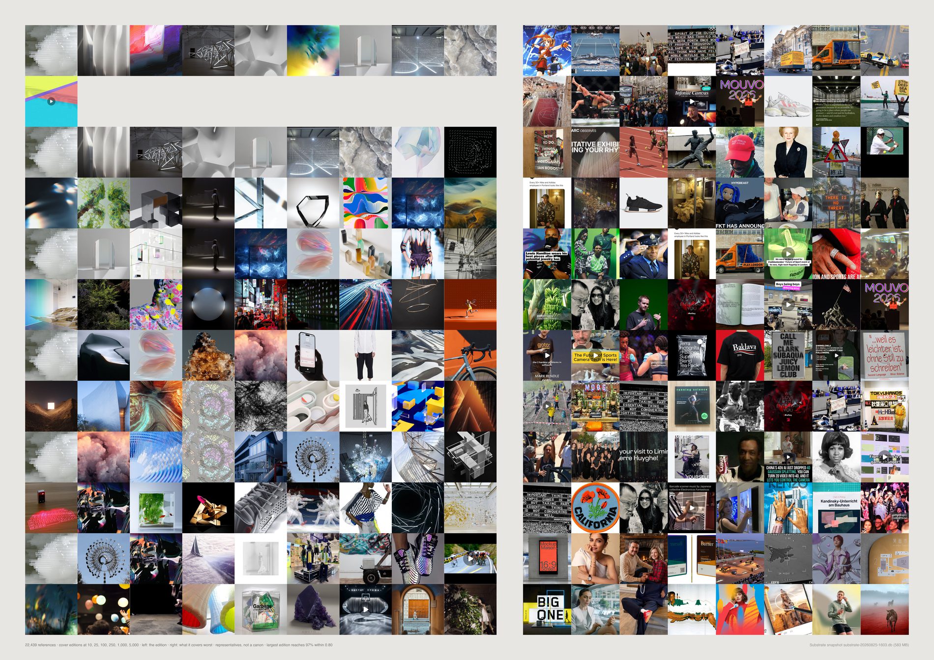
Ten images cover a third of this archive. 35.0% of 17,499 references sit within cosine 0.80 of one of ten pictures; 250 cover 63.2%; 5,000 — less than a third of the archive — cover 99.3%.
The centre is enormously compressible, which is an unflattering and useful thing to know about fourteen years of looking.
pool(), aesthetic filter on. An edition is a selection to show, so it has to be drawn from the material saved as reference. It also matters for the number itself: a large block of near-identical link cards is trivially covered by one representative, and counting them would overstate how compressible the studio's looking is. 19,209 references become 17,499.
Territories with no representative at all, of 64: 54 at an edition of 10, 45 at 25, 20 at 100, 6 at 250, 1 at 1,000. So the 100-image edition reaches 55.0% of the archive while holding nothing from 20 of its 64 regions. A small edition reproduces the centre and erases the edges.
A random draw from the 240 references that edition covers worst. Read down and the left side fills with the archive's actual material while the right side stays what it is. Even with the aesthetic filter applied, what an edition never reaches is not the archive's rarest beautiful thing.
Every method here optimises for covering the space and none has any opinion about quality. A picture chosen at scale 10 is chosen because nothing else looks like it. cover is nested, so the first cell of every band is the same picture — that is the ladder showing, not a printing fault.
What would make this wrong. “Represented” means “something within 0.8 cosine of it was kept”, and CLIP cosine is not perceptual adequacy; two pictures at 0.85 can be a photograph and a render of unrelated things. The territories are k-means regions imposed on a space that is neither round nor evenly dense — and on the filtered pool the smallest of the 64 holds just 4 references, so “lost territories” is a coarser measure here than the count suggests. Nesting is a property of cover and fps only; the kmedoid ladder is six unrelated selections.
python3 src/viz/d06_edition.py --dpi 300
# the full method comparison behind the caption:
# python3 src/viz/d06_edition.py --sweep
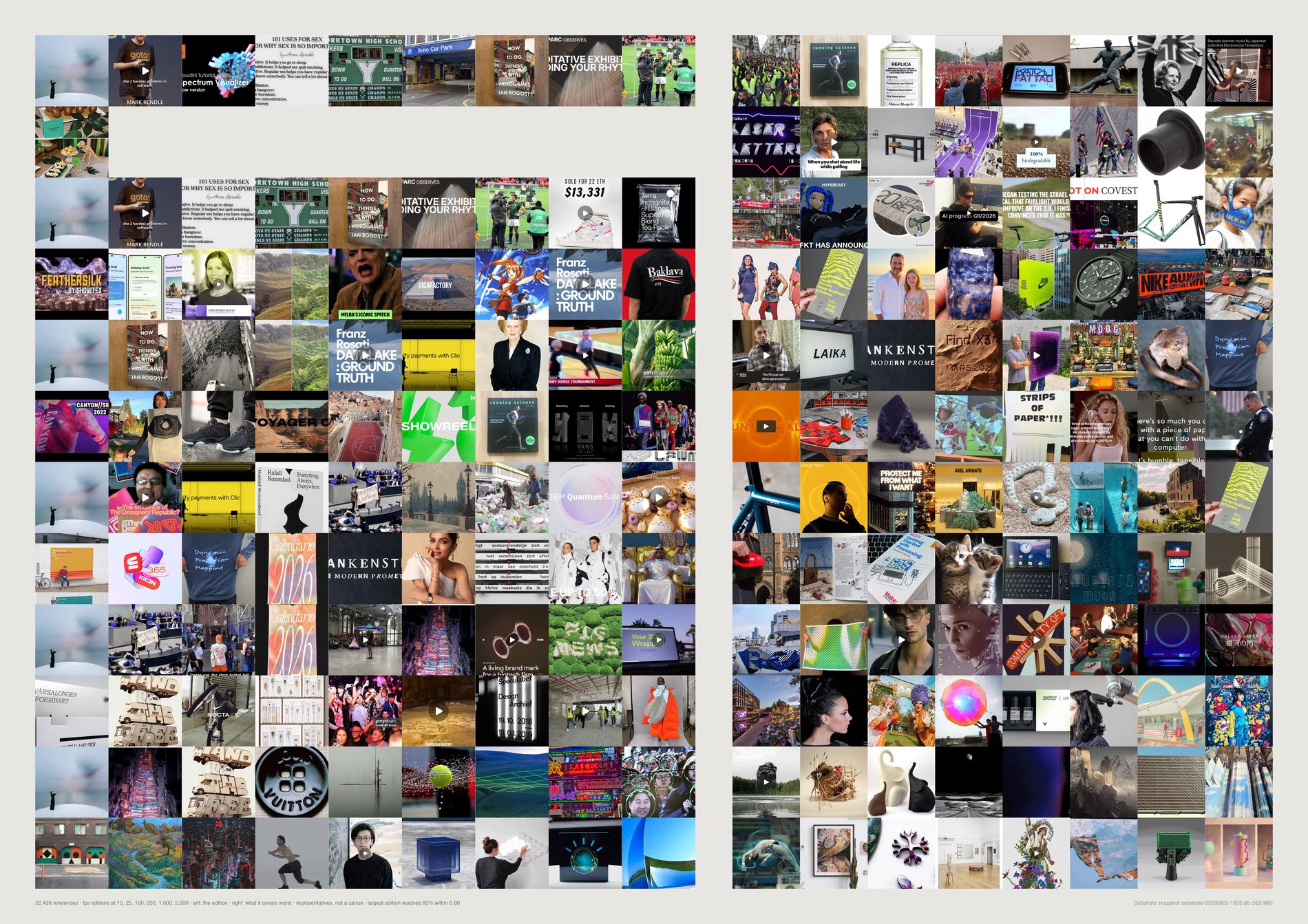
Random beats it at every scale, by a factor of seven at the small end and still by 5.8 points at 5,000.
Within cosine 0.80, fps against random: 1.1% / 7.5% at 10 · 1.2% / 18.3% at 25 · 1.7% / 35.3% at 100 · 2.6% / 43.2% at 250 · 8.1% / 60.8% at 1,000 · 75.0% / 80.1% at 5,000. Greedy set cover, at the same scales, runs 35.0% to 99.3%.
The earlier account of this failure was that fps “walks straight out to the archive's junk — screenshots of text posts, blank scans, broken thumbnails”. That explanation is no longer sufficient. This run is on the pool with those excluded, and fps still loses to random at every scale, by almost exactly the same margins. The failure is the method's, not the archive's.
Each pick is whatever is currently worst covered, so the set grows outward from the edges inward and spends the entire edition on outliers. Inferred: what fps finds when the screenshots are gone is simply the next most isolated material — which is still, by construction, the material that represents least.
The swell figure — the largest ratio between a region's share of the edition and its share of the archive — runs x33.3 at 100 and x12.8 at 1,000 for fps, against x2.8 and x1.9 for cover. Read it from 100 upward; below that it is dominated by granularity rather than by bias.
It is worth printing precisely because it looks wrong. This is what “maximise diversity” means when it is applied literally to a real archive, and it is the standard answer to the question this direction asks.
What would make this wrong. Coverage at cosine 0.80 is one figure of merit and it is the one cover optimises directly, so the comparison is not neutral between the methods — a set-cover method winning a set-cover metric is close to a tautology. The result that survives that objection is fps against random, which optimises nothing. Note also that fps closes most of the gap at 5,000 (75.0% against 80.1%), so this is a failure at small edition sizes, not at every size.
python3 src/viz/d06_edition.py --method fps --dpi 300
Direction 07. Which findings survive the method
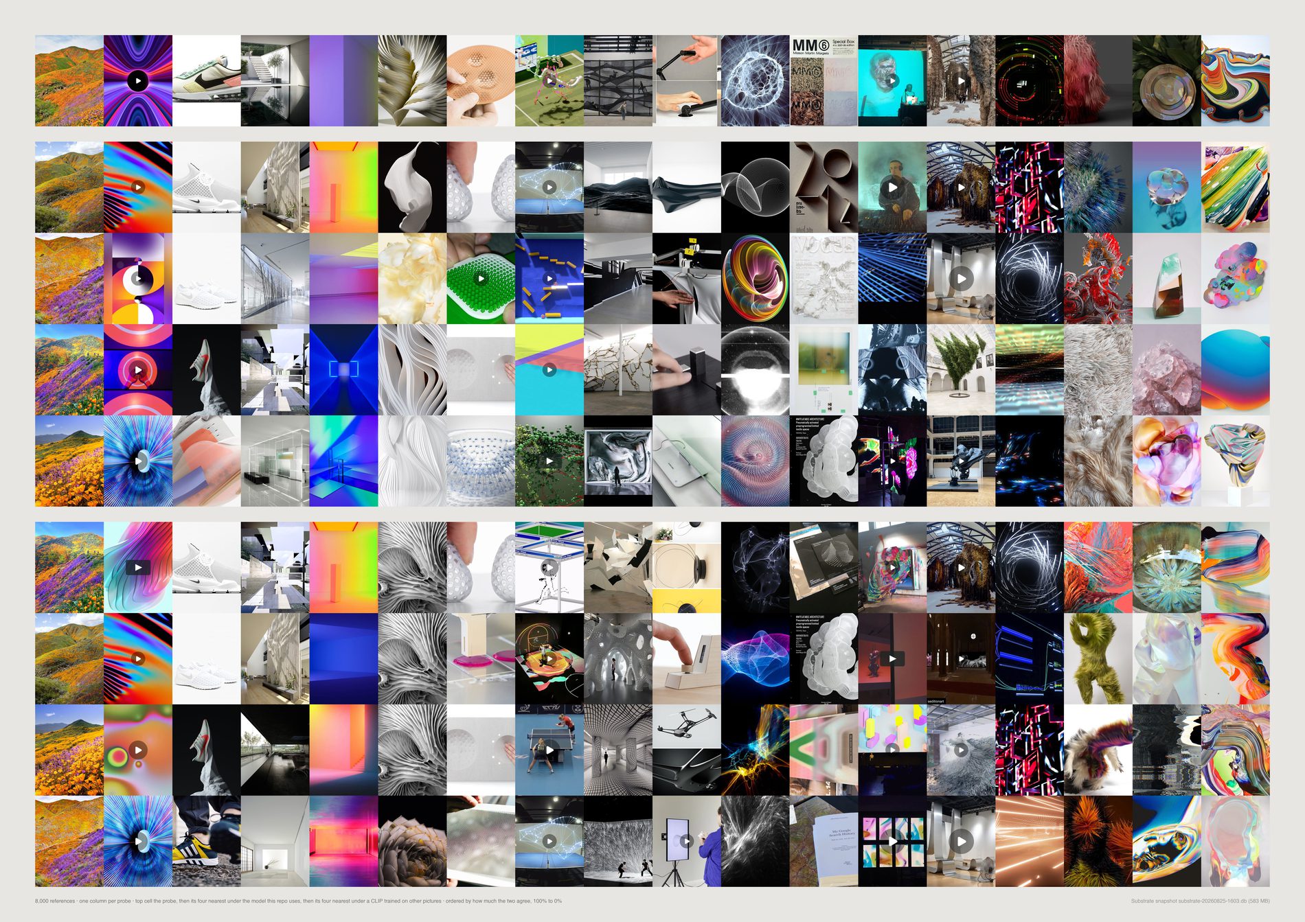
The cluster structure survives everything. AMI against FIELD's own boards holds at 0.160–0.162 across five seeds (between-seed ARI 0.76), 0.170 on a CLIP trained on entirely different pictures, and 0.143–0.176 under four surgeries — the pool filters removed, Pinterest removed, the largest board removed, board-balanced sampling.
It is the strongest finding in the project and it is now stronger.
The loneliness result survives everything. Two definitions of “alone”, zero overlap in their top 48, at k = 4, 8 and 16, on both models. Six measurements, six zeros. That disagreement is a property of the archive, not of a parameter.
Board coherence's numbers are a fact about one model. 0.713–0.843 on OpenAI CLIP against 0.532–0.714 on LAION — the whole range shifted down by about 0.18. The ranking is safe (cross-model rho +0.94, split-half rho +0.88 ± 0.02), so “Culture is the loosest board in the archive” holds. “Board coherence runs 0.71 to 0.84” must never be quoted without the model beside it.
Median cluster purity is not a number at all. 0.10 to 0.11 across seeds; 0.06 to 0.55 across the inclusion rules. Cap every board at 60 references and it is 0.06; remove Pinterest and it is 0.55. An order of magnitude, from choices nobody would think to write down. Purity should be reported with its inclusion rule or not reported.
No 2-D map of this space can support the claim a reader makes of it. A PCA plane keeps 2.3% of a reference's ten nearest neighbours. t-SNE keeps 29.0% — far better, and still seven of ten neighbours on the page are not the neighbours — and two t-SNE seeds of the same data agree with each other on only 55.4% of what they each draw. A 2-D atlas can support “there are regions and here is roughly where they sit”. It cannot support “these two things are near each other”.
“Similar” is model-specific, and not marginally. Two CLIPs of identical architecture differing only in training corpus return the same top-10 neighbourhood 33.5% of the time. The control that makes that readable: the same model asked over half the archive returns 100% the same neighbours, so the 33.5% is the model and not the noise. Substrate's own text vectors agree with the image vectors 2.7% of the time and eight non-learned measurements 1.7% — above a chance rate of about 0.05%, and useless.
pool(), aesthetic filter on, through src/d07_reps.usable_refs. This one is forced rather than chosen: the findings being audited — clusters.py, coherence.py, loners.py, flex.py, atlas.py — are all computed on the pool. An audit run on a different population is not an audit, it is a sixth answer. 19,209 references become 17,499; 16,499 of them carry all four representations.
It is to say which questions this material can answer and which it only appears to answer. A finding that survives four representations is worth more afterwards than it was before; one that does not needs saying out loud, and four here do not.
One column per probe, ordered by cross-model agreement. Top cell is the probe, then its four nearest neighbours in this repo's model, then its four nearest in the other one. On the left the two blocks are the same pictures. Somewhere across the page they stop being the same pictures. That is the finding rendered rather than plotted: the archive is real, its neighbourhoods are constructed.
This repo's own numpy k-means is verified against sklearn's on the same data: inertia 6,098 to 6,098. That check exists because a convergence bug here once returned unfitted k-means++ seeding and produced a false null in direction 09.
What would make this wrong. Two CLIPs are not two models — same architecture, same objective, same rough era — so agreement between them is evidence against a corpus artefact and nothing stronger. The text and measured representations are included precisely because they are not CLIP, and they disagree with it far more. A moved number is not a wrong number: board coherence on another model is a different measurement, not a correction of the first, and the claim under test is only ever “would the sentence in the docstring still be written”. The surgeries are not independent — removing Pinterest removes most of the archive's colour, dates and boards at once. And t-SNE runs on a 4,000-reference subsample, because the question (do two seeds agree) is answerable at that size.
python3 src/viz/d07_stability.py --dpi 300
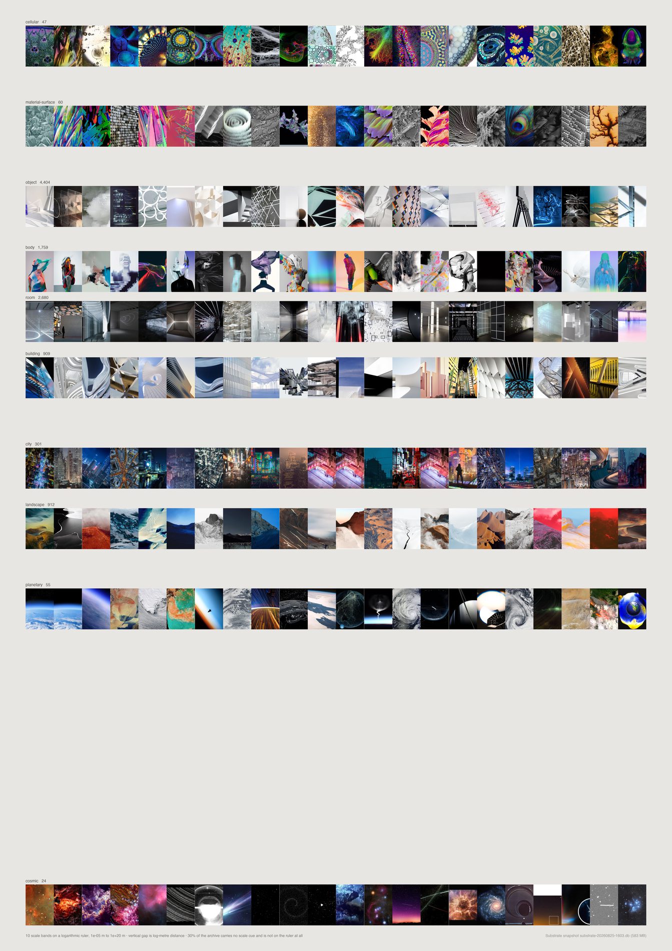
Scale-indeterminate is the largest band in the archive: 5,782 references, 33.3%. The vision pass returns a scale band and the cue it used, and where the cue is none the record is forced to indeterminate at parse time rather than believed.
So a third of what this studio collects is material an eye cannot put a size to.
Of the 11,584 that do carry a cue, the mass sits in four adjacent bands — object 4,608 (26.5%), room 2,714 (15.6%), body 1,855 (10.7%), landscape 944 (5.4%). That is 58.3% of the pool inside roughly 0.1 m to 10 km. Human and near-human scale.
The two ends the direction is named after are close to empty. Molecular 5, cellular 48, material-surface 60, planetary 62, cosmic 30 — 205 references, 1.2% of the pool across both extremes combined. Molecular does not clear the twenty-image floor and is not drawn at all.
The gap between two bands is proportional to the log-metre distance between them, so the crowding near a metre is the archive's own crowding and the long empty runs are decades nobody looks at. Within a band, images run by cosine distance to that band's CLIP centroid — most typical first.
Default pool. This is a question about what the studio looks at, and the headline number is the indeterminate band. A link card or a screenshot of a chart has no depicted scale and lands there by construction, so counting them would be counting the answer into the question. 1,812 references dropped, and indeterminate fell from 36.0% to 33.3%.
The log positions are order-of-magnitude stand-ins chosen so the ruler can be drawn. “Room” is not 5 m in general. cosmic at 1e20 m is the worst of them and it dominates the page: half the sheet is the gap beneath it, which is truthful about astronomy and arbitrary in its exact size.
What would make this wrong. The cue column is the model's claim about its own reasoning, which is weaker than a record of it — a model can report human-figure on an image with no figure, and nothing here audits that. A recheck over 500 images asked twice puts scale at 90.8% and the cue at 91.6%: stable, which is not the same as right. And indeterminate is doing two jobs — an abstract gradient genuinely has no scale, a tight crop of a building has one this image cannot show, and both land in the same band.
python3 src/publish.py d11-scale-ruler
# python3 src/viz/d11_scale.py --page a2 --dpi 300
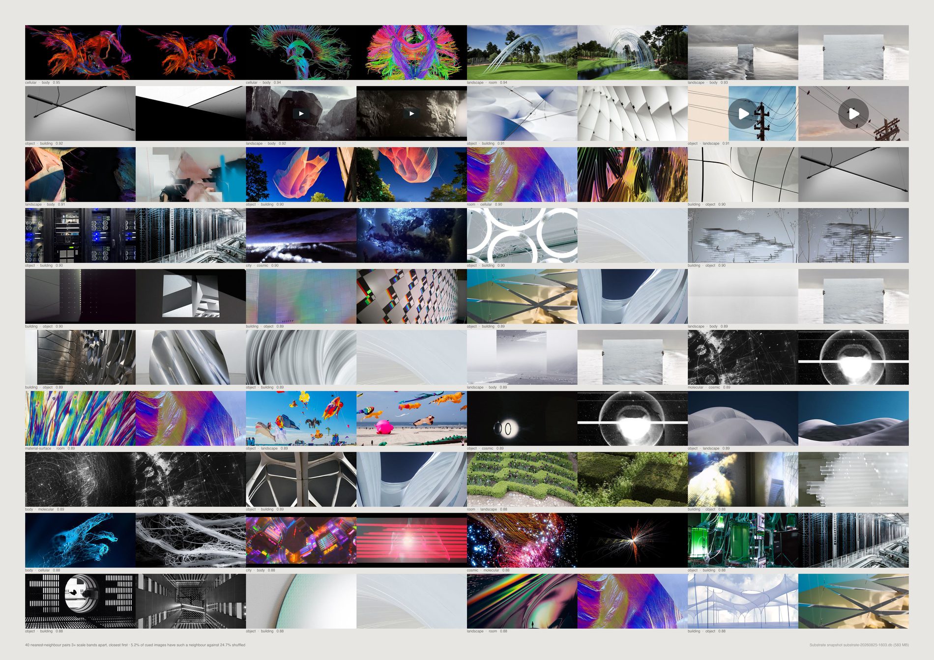
Take every reference with a real scale cue, find its nearest CLIP neighbour, and ask how often that neighbour is three or more bands away. 5.42%. Shuffle the bands and the same count is 24.84%.
A ratio of 0.22: images that look alike here are about a fifth as likely to cross scale as chance would put them.
Visual similarity in this archive is strongly scale-preserving, which is the inverse of the direction's hypothesis, not a weak version of it.
The pairs that do cross are real and there are not many. Cellular against body at 0.949 cosine, landscape against room at 0.936, landscape against body at 0.933. One of the closest pairs was dropped as a perceptual duplicate — the same picture labelled two ways, which is a model inconsistency wearing a wormhole's clothes.
A duplicate pair scores 0.99 cosine and crosses three bands, so it would sit at the very top of this sheet as a labelling error rather than a finding. It stays in the 5.42% because there the shuffled baseline controls for it. Near-duplicates are caught at Hamming distance under 6 on the 64-bit pHash.
Forty pairs out of a pool of 17,359. The direction's idea works — it is just rare rather than characteristic, and a sheet of forty is the entire population of it above this similarity floor.
What would make this wrong. Both bands in a pair are the model's, so a wormhole can be a mislabelling in either direction, and the shuffled baseline cannot tell those apart from real ones. The rate is also sensitive to the three-band gap: a two-band gap counts “object next to body” as a crossing, which it plainly is not.
python3 src/publish.py d11-wormholes
# python3 src/viz/d11_scale.py --wormholes --page a2l --dpi 300
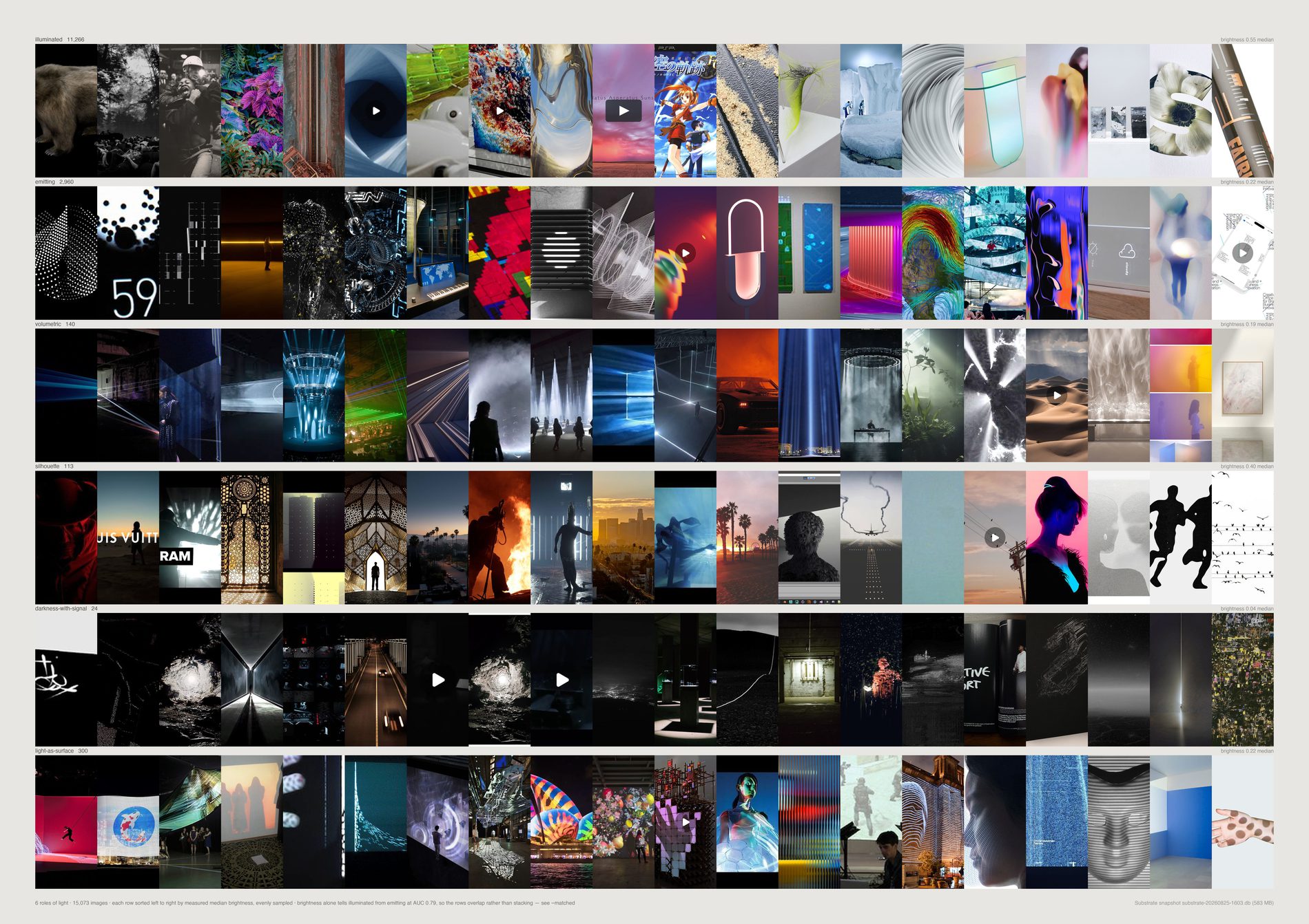
The distribution is lopsided in a way worth saying out loud. 72.8% is the ordinary case — light falling on a subject, 11,902 references.
21.6% is a subject that is itself a light source: 3,530 references of screens, neon, LED, projection and glowing form.
Everything the direction is most interested in is together under four per cent. Light-as-surface 302 (1.8%), volumetric 140 (0.9%), silhouette 123 (0.8%), darkness-with-signal 27 (0.2%) — 592 references, 3.6% of the pool.
Emitting at better than one image in five is the number that carries the story. Screens and glowing form are not a minor register here; they are the archive's second subject. Their median brightness is 0.22 against illuminated's 0.55, which is physics rather than a labelling artefact: a light source is usually photographed against a dark surround.
Default pool. A question about what light is doing is a question about taste, and a screenshot of a web page is lit by nothing. 1,784 references dropped from the 18,144 that carry both a perception record and a photometric measurement.
The brief's interesting story is a progression over fourteen years from light as treatment to light as material. Substrate has three date columns and none of them is “when FIELD found this” for more than about a tenth of the archive. A curve drawn on created_at would be a curve of when other people posted things, so it is not drawn and the progression stays open.
A frame can be a silhouette against a volumetric beam. The model returns one label, the rows are not a partition of anything, and a picture doing two things is filed under one.
What would make this wrong. darkness-with-signal has 27 references in sixteen thousand. Its row is a handful of pictures, not a register, and the counts print on the sheet so a thin row cannot pass as a thick one. The recheck is stability rather than accuracy: light_role comes back the same on 93.4% of 500 images asked twice, but light_source only 83.6%, which is why the source cut is the weakest of the three.
python3 src/publish.py d12-light-role
# python3 src/viz/d12_light.py --field role --page a2l --dpi 300
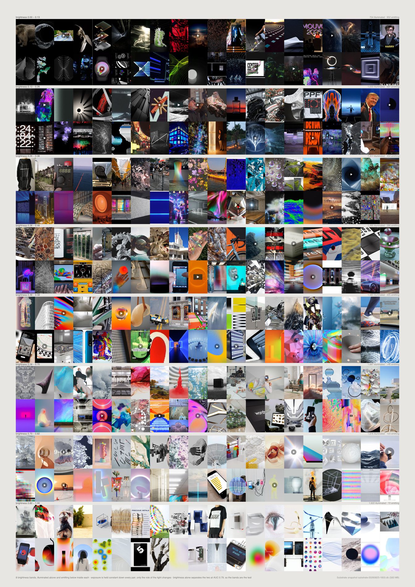
The guardrail asks that brightness not be treated as meaning. The obvious way to satisfy it is to show that brightness does not predict the roles.
It does. Median brightness separates illuminated from emitting at AUC 0.775, a long way from the 0.5 of a number carrying no information.
So the claim “these families are not exposure” would have been false, and an uncontrolled version of this piece would have printed it.
What is drawn instead holds exposure fixed. Eight brightness bands; inside each, a row of illuminated above a row of emitting. Down every pair the pixels are equally bright and only the role changes — and the two halves still look nothing alike. In the bright bands the emitting half is screens, interfaces and colour fields while the illuminated half is objects and interiors. Not “brightness is irrelevant”, but “the role survives brightness being held fixed”.
These groups are 77/23, so “always say illuminated” scores 77.1% while knowing nothing at all, and a threshold adds 2.8 points on top without the number carrying much. AUC is the probability that a random member of one group outranks a random member of the other, and 0.5 is no information regardless of how lopsided the classes are.
Entropy 0.624, median saturation 0.584, brightness spread 0.549. The one photometric number that works is the obvious one, and it works by about the margin physics predicts.
Emitting is front-loaded into the dark end — 1,141 against 730 in band one, 110 against 1,662 in band eight. The rows are sampled evenly through each cell of the matrix, so the sheet argues about what the two kinds of frame look like at equal exposure and never about how many of each there are.
What would make this wrong. Four photometric numbers tried one at a time is not every photometric number. A trained classifier over all of them, or a feature closer to what “emitting” means — the shape of the top percentile of the histogram, say — would likely beat 0.775. That still would not make the labels meaningless; it would mean the model is naming something a photometer can partly see, which is what one would expect.
python3 src/publish.py d12-light-matched
# python3 src/viz/d12_light.py --matched --page a2 --dpi 300
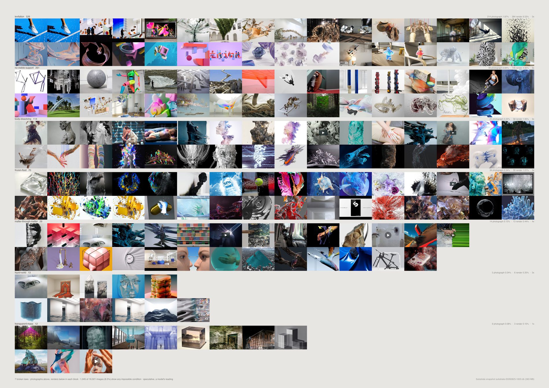
6.41% of the pool shows any impossible condition at all — 1,039 references. The rest is none.
Whatever this studio's relationship with physics is, it is not that most of its references break it.
Two conditions carry most of it: levitation 519 and no visible support 258, which are close to the same observation made twice — an object in the air, and an object that ought to fall. They should probably be read as a single count of 777, 4.8%. Third is body-dissolving-into-field at 119, fourth frozen fluid at 68. Everything else in the brief's list is in the low tens or fewer: matter-through-matter 28, liquid-solid 13, impossible-scale 13, transparent mass 12, sideways gravity 7, endless depth 2.
What the impossible images are of: abstract 22.0%, installation 16.7%, person 11.7%, object 11.3%, sculpture 10.2%.
The brief calls human review essential and it has not happened. What the repo can do instead is put every image on the page beside its claimed law at a size where a reader can reject it. The blocks are visibly coherent, which is itself some evidence the labels mean something, and it is not review.
Raising the floor changes almost nothing: 1,039 at conf ≥ 0, 1,039 at conf ≥ 2, 987 at conf ≥ 3. The model answers 3 nearly every time it answers at all. impossible_conf is 97.6% stable across a recheck, which is stability without content, so it filters nothing here.
Default pool. The medium control divides photographs from renders, and the non-aesthetic material — link cards, pure typography, screenshots — is labelled graphic or illustration rather than either, so leaving it in dilutes both denominators and moves every lift. 1,783 references dropped.
What would make this wrong. The condition label is the model's poetic reading, exactly as the guardrail warns, and it is the most stable field in the pass at 96.6% over 500 images asked twice — which is still not review. The medium label is also the model's, and a photograph of a screen showing a render is a photograph; the lift column inherits that error in the direction that inflates the finding.
python3 src/publish.py d13-impossible
# python3 src/viz/d13_impossible.py --page a2l --dpi 300
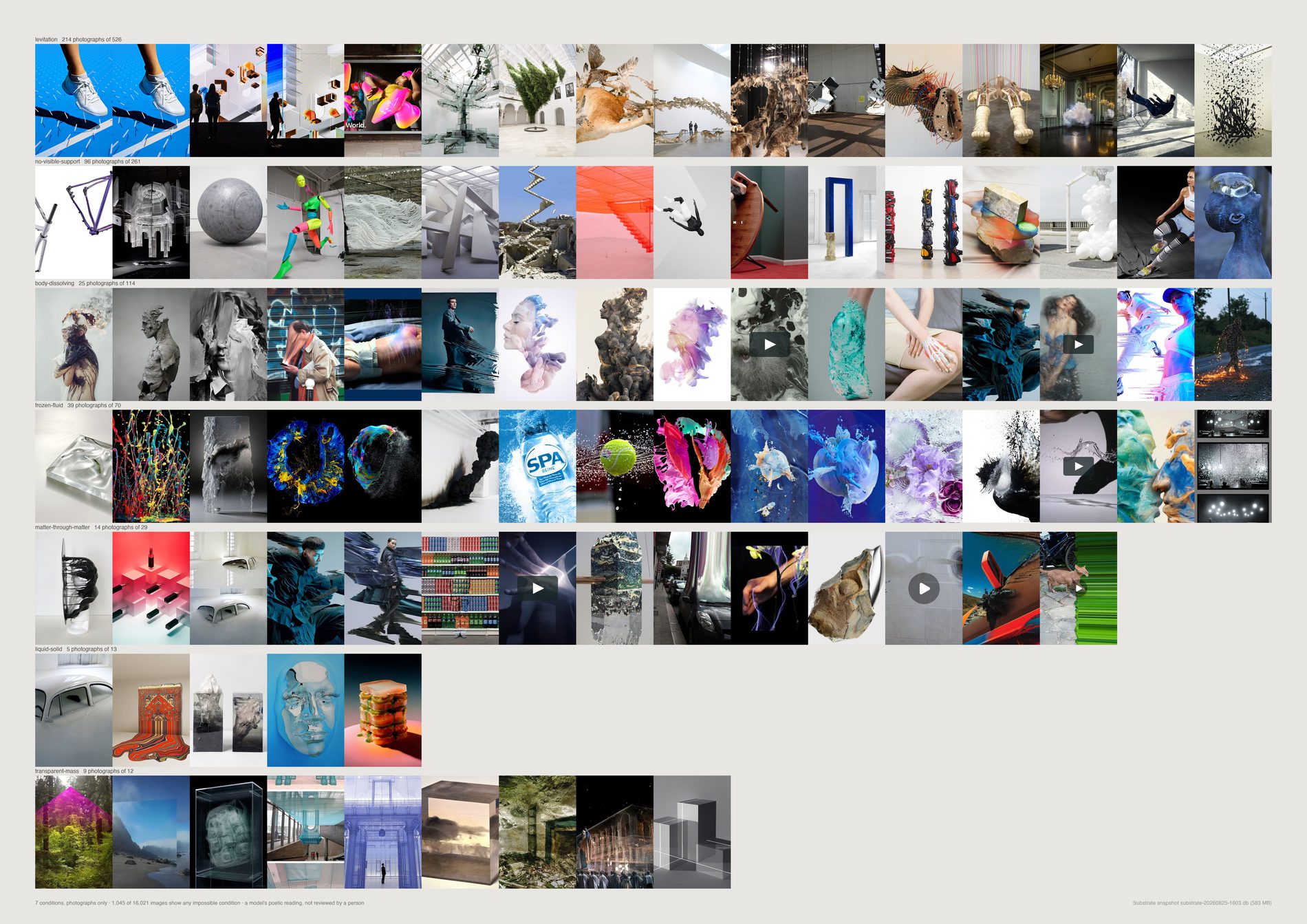
The pool is 65.2% photograph against 27.1% render. A render can break physics for free; a photograph mostly cannot, and when it does someone built a rig, waited for a splash, or lied in post.
So a count of impossible conditions with no medium control is a CGI detector wearing a poetics costume.
Measured: photographs 3.43%, renders 14.14%, an overall lift of 4.1×. The warning in the brief was right, and the uncontrolled version of this piece would have ranked a taste for the impossible by how much 3D work the studio happens to have saved.
What survives the control is small and specific. Two conditions have a lift near 1, meaning the medium does not explain them — transparent mass at 1.4× and sideways gravity at 1.8×, both tiny at 12 and 7 references. The one with both a low lift and real weight is frozen fluid at 2.7× over 68 references: splashes, suspended liquid, a pour stopped mid-air. Endless depth is the only condition that appears exclusively in photographs, and it has two.
So the direction does not support “FIELD repeatedly seeks worlds where physical rules become negotiable” as a measured claim about the archive. It supports a much narrower one about frozen fluid.
How many times more often a render shows a condition than a photograph does. High lift means the condition was made. Near 1 means it was sought, and those are the only ones this direction can honestly claim.
Once inside each medium, on the same population, so the control denominator and the catalogue numerator can never drift apart. That is why the pool filter had to be applied before the split rather than after.
What would make this wrong. Transparent mass at 12 references and sideways gravity at 7 are the two results that survive the control, and neither is a population you can conclude anything from. The honest reading of this sheet is that the control removed the finding and left a hypothesis worth testing on more material, not that a smaller finding was recovered.
python3 src/publish.py d13-impossible-photographs
# python3 src/viz/d13_impossible.py --photographs --page a2l --dpi 300
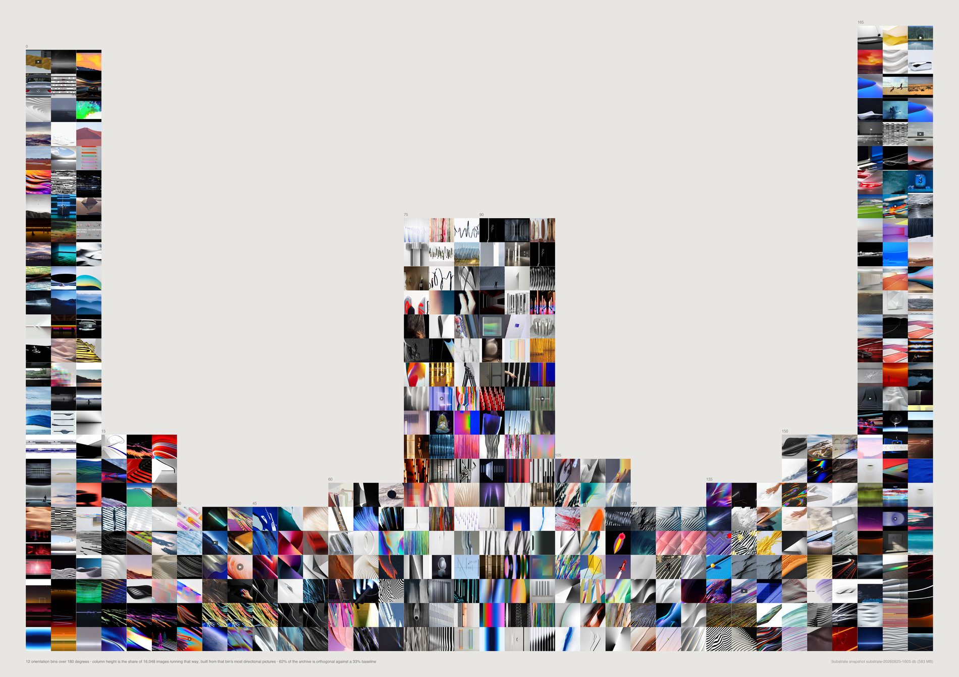
36.3% of the pool has a dominant axis within fifteen degrees of horizontal — 3,111 in the first bin and 3,200 in the last, against a 16.7% baseline for those two bins together.
24.8% is within fifteen degrees of vertical, against the same 16.7%.
Together: 61.1% of the archive is orthogonal against a 33.3% baseline. That is a strong, real measurement, and it is what horizons, skylines, table edges, window ranks, columns of type and the rectangle of the frame itself produce. It is almost certainly not about motion.
And the pixels cannot detect motion at all. Median coherence of frames the model calls still is 0.215; of frames it calls moving, 0.231. Directional structure does not distinguish the two. The radial fit is worse than null — 0.070 for still frames against 0.063 for the ones labelled radial, the wrong way round.
The obvious suspicion is that the orthogonal peaks are screenshots and pages of type, which are the most perfectly orthogonal objects in any archive. The default pool removes 1,816 references and the towers barely move — 62% orthogonal before, 61.1% after. So the frames are the archive's, not the filter's leftovers.
Its bin's own most directional images, most coherent at the bottom. Which is close to circular for the towers: the columns select for streaks and strong parallel structure, and coherence is what measures those. The thousands beneath the drawn cells are counted and not drawn.
Median 0.217 of a possible 1.0, ninetieth percentile 0.545. Direction 14's premise — that this studio selects stills already carrying behavioural potential — is not what the archive says. It selects stills.
What would make this wrong. A still image has an axis and never an arrow. Rising and falling are the same measurement to a structure tensor, and the sign exists only in the model's answer. Orientation from gradients is objective and measures the wrong thing — a brick wall scores as a strong horizontal — which is the whole reason both readings are on the page instead of one.
python3 src/publish.py d14-wind-map
# python3 src/viz/d14_latent_motion.py --page a2l --dpi 300
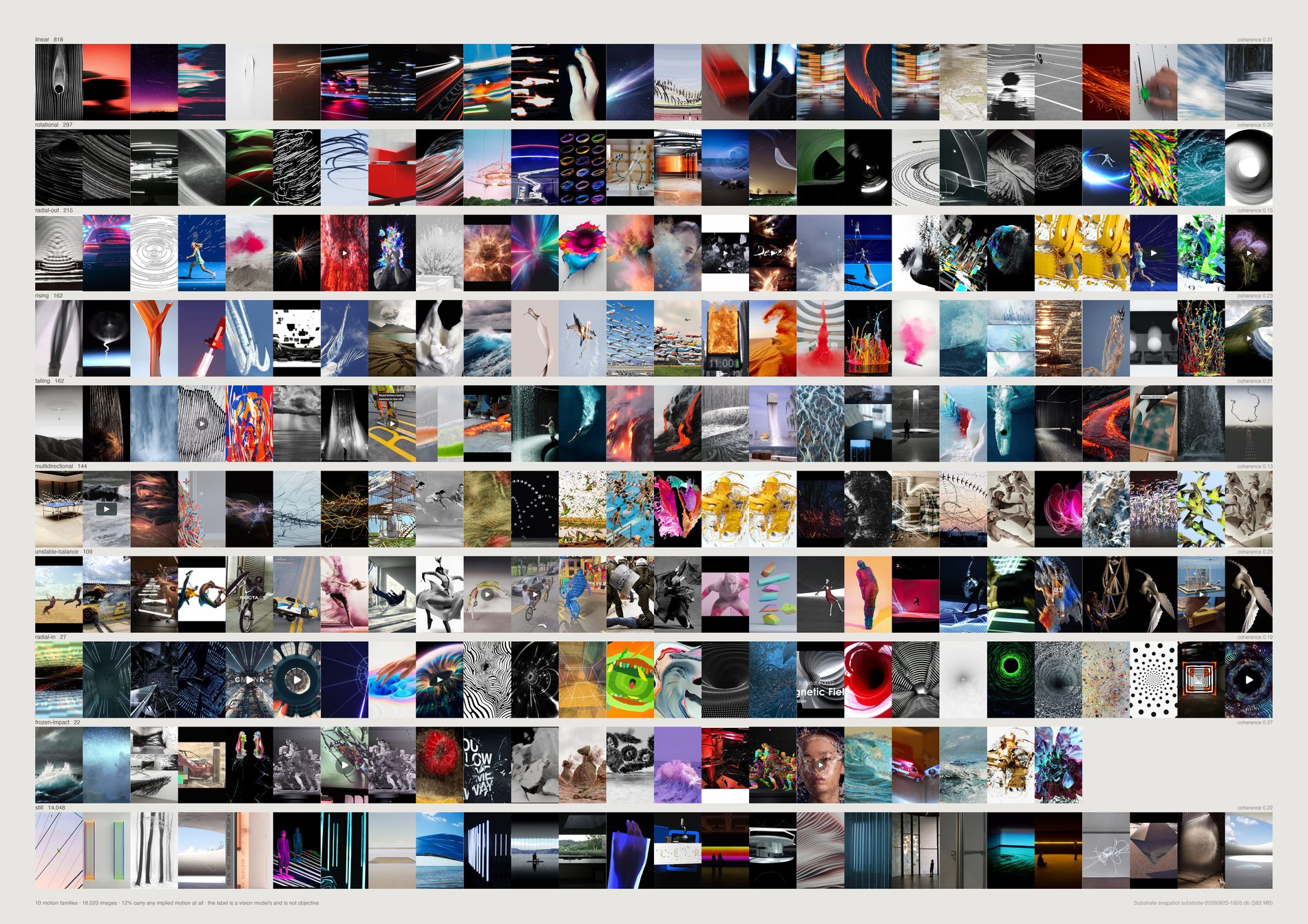
The archive is still. 15,248 references come back still — 87.8%. Counting indeterminate as well, only 12.1% carries any implied motion at all, and the largest moving class is linear at 868 (5.0%).
The one genuine positive is the agreement test. Of the 867 references the model calls linear and gives a direction, 54.4% have a pixel axis within thirty degrees of it against 33.3% by chance, with a median error of 22.5° against 45°.
That is far outside noise. When the model says an image moves left to right, the gradients agree that it runs left to right — two independent methods, one made of arithmetic and one of language, landing on the same angle.
Falling holds up at 51.2% over 172; rising does not, at 40.9% over 171 with a median error of 42.3°.
So the pixels can confirm a direction the model reports and cannot detect motion the model reports. Those are different claims and the sheet keeps them apart.
linear at 0.313 median against the archive's 0.215. Which is close to circular: a linear-motion image is largely defined by having a streak in it, and a streak is what coherence measures. The vortex fit is the only other positive — 0.103 for the 322 rotational frames against 0.073 for still ones, weak.
Rising and falling collapse to vertical for the comparison because a structure tensor has no sign. Scoring the model mod 360 would be scoring it against a number that does not exist.
The prompt offered still as a correct and common answer, which is honest and also makes it the cheap answer. The motion label is 95.8% stable over 500 images asked twice; motion_conf only 76.8%, so the confidence field filters nothing here.
What would make this wrong. Neither reading is trustworthy alone, and the agreement test is the only ground they share. It can only be run on the three labels that name a direction — 1,210 references of 17,358 — so the positive result covers seven per cent of the material the sheet draws.
python3 src/publish.py d14-motion-families
# python3 src/viz/d14_latent_motion.py --families --page a2l --dpi 300
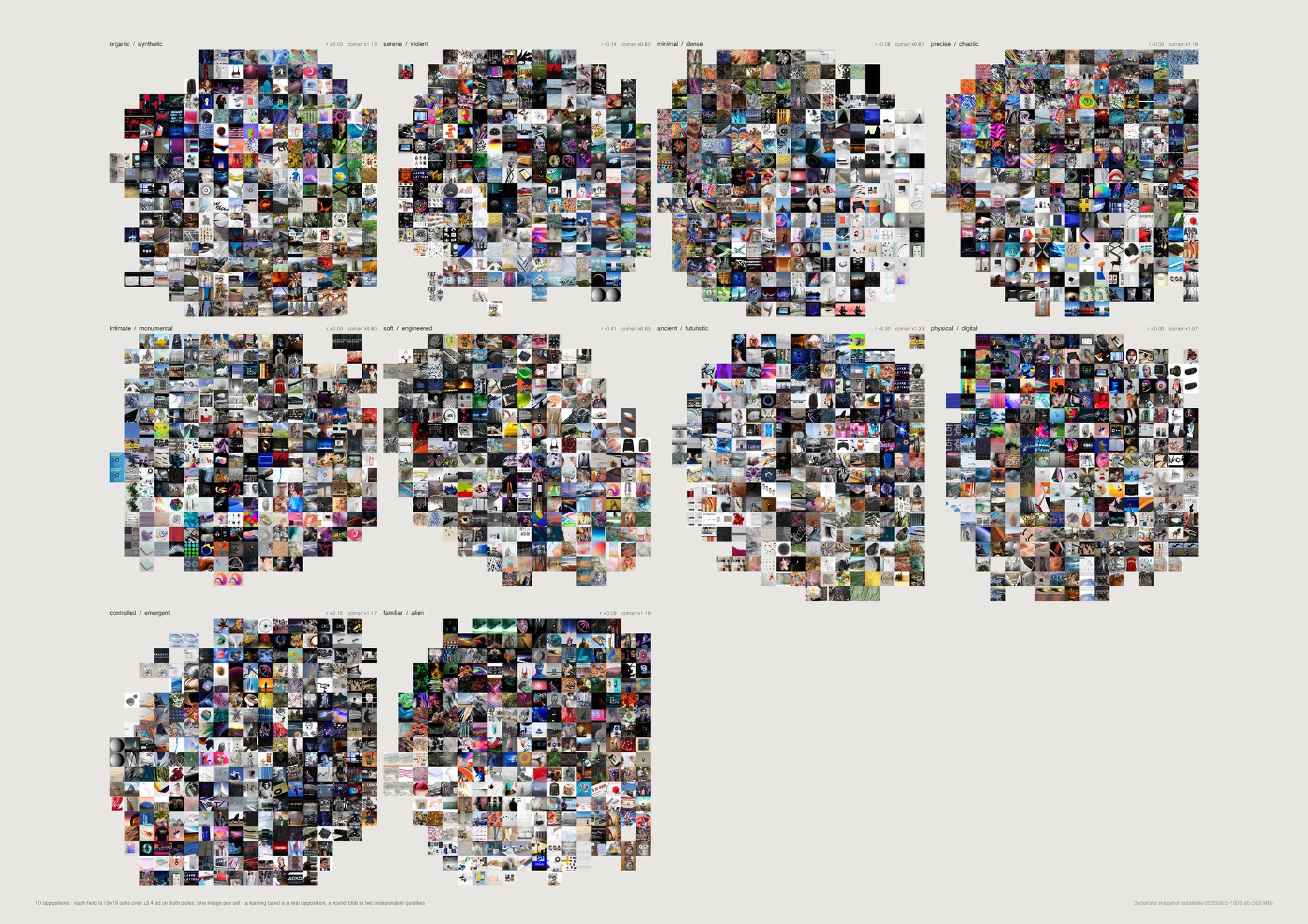
Of the brief's ten oppositions, exactly one behaves like a strong opposition in this archive: soft/engineered at r = −0.409. Three are weak — ancient/futuristic −0.184, serene/violent −0.131, minimal/dense −0.080.
The other six are not oppositions at all. Precise/chaotic −0.073, physical/digital −0.002, intimate/monumental +0.009, organic/synthetic +0.046, familiar/alien +0.091 — and controlled/emergent comes out positively correlated at +0.158, meaning the two words describe the same images here.
And the corner is not over-populated. Excess — the count of double-high images against what each axis's own correlation predicts — runs 0.79 to 1.24 across the ten.
Nothing near a doubling. Only ancient/futuristic at 1.24 and familiar/alien at 1.18 sit above the noise, and neither by enough to claim.
So the archive does not demonstrably over-collect images that hold opposing qualities. What it shows instead is that most of the proposed oppositions were never oppositions — the guardrail's own question answered rather than the brief's.
Scored the obvious way, with no debiasing, all ten axes came out positively correlated at r between +0.55 and +0.83 — which reads as “every one is a false binary”. That was CLIP's text cone, not FIELD. The gap between those two runs is the largest single effect measured anywhere in this direction, and it was produced entirely by the method. It is why the numbers print on the sheet rather than being summarised.
Quantile bins fill the square evenly and would hide the very thing the field is drawn to show — that a real opposition leaves its top-right corner empty. Occupancy runs 75% to 87% of 324 cells, and soft/engineered is the emptiest at 75%.
Default pool, and every statistic recomputed over it rather than inherited. d15_poles.py scores the whole embedding set with only the duplicate filter, because encoding CLIP text directions is the expensive half. Here the z-scores are re-standardised over the 17,522 that survive the pool and r and the corner excess computed again from those — otherwise a correlation measured on one population would sit beside cells drawn from another.
What would make this wrong. CLIP's word is not the studio's word: “monumental” is trained largely on captions about buildings, so an axis can sort subject matter while appearing to sort quality. And absence of excess is not absence of contradiction — this measures contradiction as two text directions both scoring high, which is a thin proxy for an image that genuinely sustains two readings. A picture can be unmistakably both serene and violent to a person and score unremarkably here.
python3 src/publish.py d15-field-contradictions
# python3 src/viz/d15_contradictions.py --page a2l --dpi 300
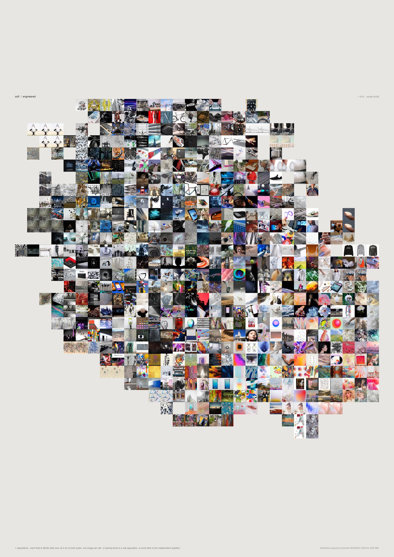
r = −0.409, the only strong opposition among the brief's ten, and the field leans as a diagonal band because scoring high on one pole really does cost you the other.
Its corner — both poles above +1 sd — holds 93 references, which is 0.53% of the pool against the 0.64% that this axis's own correlation predicts. An excess of 0.83: emptier than chance, not fuller.
The axis is about making, not about mood. Asked to propose its own pairs rather than take the brief's, the archive returns natural/machinic (−0.49), soft/machinic (−0.46), soft/industrial (−0.42), organic/machinic (−0.39). The recurring pole is machinic, and the tension these references hold is hand-and-body against machine — not serene against violent, and not any of the temporal or scale pairs.
The corner's own subject mix backs that: product 24%, object 15%, person 9%, and 73% photograph.
68% occupancy against 75–87% for the others. A real opposition cannot fill its corners, so the empty paper is the measurement rather than a gap in the data.
A cell holding four hundred candidates and a cell holding one look identical on the page. The counts print to stdout; the picture does not carry them.
What would make this wrong. The ten pairs are the brief's guess and the search bank is mine — neither is the studio's vocabulary. Every pair in this piece is a proposal a person should accept or throw out, and the fact that the archive's own best axis is natural/machinic rather than anything the brief named is the clearest sign the vocabulary came from outside.
python3 src/publish.py d15-field-soft-engineered
# python3 src/viz/d15_contradictions.py --axis soft/engineered --page a2 --dpi 300
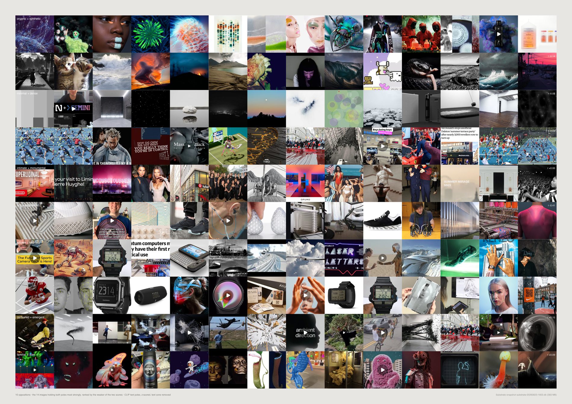
Depth is the largest guaranteed score on the weaker pole. Ranking on the sum would let a huge left score carry a mediocre right one, which is the opposite of what a contradiction card wants.
Corner populations run from 93 (soft/engineered) to 696 (controlled/emergent). The subject mixes are the honest reading of them:
intimate/monumental, 355 references — person 18%, interior 16%, installation 14%, and 90% photograph. Ancient/futuristic, 334 — architecture 22%, product 15%, and 46% render, the most render-heavy corner on the sheet. Controlled/emergent, 696 — installation 25%, abstract 15%, which is the corner of a pair that was not an opposition to begin with.
A corner that is 80% one subject found a category, not a tension. None of these are that concentrated — the strongest is installation at 25% — which is mildly reassuring and not a result.
Every one of these corners is at or below what its axis's own correlation predicts. The rows are worth looking at; they are not evidence that the studio seeks the images in them.
What would make this wrong. This is a visual study and it is labelled one deliberately. The corners exist for every axis including the six that are not oppositions, so a beautiful row here is not evidence of a contradiction — for those six it is just the far end of two independent qualities, which any pair of numbers has.
python3 src/publish.py d15-contradiction-cards
# python3 src/viz/d15_contradictions.py --cards --page a2l --dpi 300
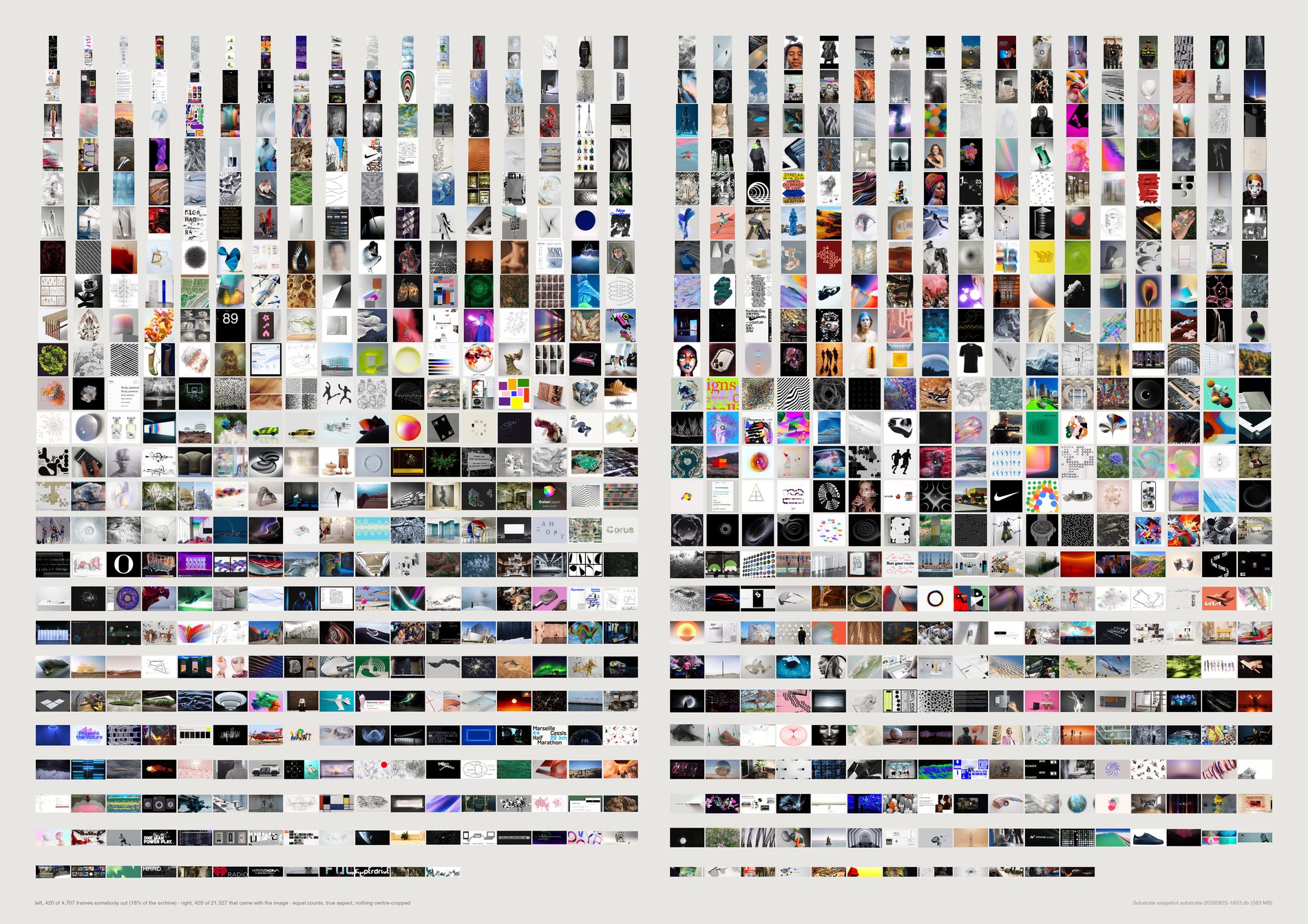
Where this studio crops, it is extracting, not reframing. Compare the 3,996 hand-cut frames carrying a vision label against the 13,142 machine-shaped ones that do, one two-proportion z-test per label:
data-visualisation 6.88% cut against 4.17% (z +7.0) · sculpture 7.36% against 4.86% (z +6.1) · made = drawing 8.51% against 4.41% (z +10.1) · made = diagram 3.38% against 1.48% (z +7.6).
And in the other direction: person 6.18% against 7.43% (z −2.7), texture 4.03% against 5.04% (z −2.6), machine 1.20% against 1.89% (z −2.9), photograph 58.56% against 61.59% (z −3.4), render 20.80% against 24.88% (z −5.3).
Measured off the pixels rather than the labels, the cut set is brighter (median 0.5412 against 0.4804) and less saturated (0.1094 against 0.1392) with more edges (0.1884 against 0.1752) — the signature of a white page with a diagram on it.
So cropping here is an act of extraction: pulling a chart, a drawing or an object off the page it was printed on.
It is not the act the brief imagined, of reframing a photograph to remove people or context. People go slightly down in the cut set. The studio takes photographs the shape it finds them.
The brief says do not assign intention when the platform created the crop — and on this material the platform created most of the crops, so it cannot be honoured by a footnote. frame_origin() splits every reference by where its proportions came from before anything is drawn.
By source, cut rates run instagram 2.4% (the platform enforces the shape at upload), manual 14.4%, creativeapplications 19.1% (a WordPress theme crops every header to 3.545:1), pinterest 28.2%, basecamp 34.5% (files a person dragged into a project thread). Instagram at the bottom and Basecamp at the top are the two ends the method predicts before looking.
The right-hand field is three times the left in reality. Drawn at true proportion the eye reads the density difference and stops looking at the pictures, and that difference is already in the caption. Both fields draw 420, sampled evenly through each set after sorting by aspect. The sheet argues about what is inside the two kinds of frame, never about how many there are.
What would make this wrong. The modal test is a threshold and 40 is a choice; --modal-min moves it and the counts move with it, which is why both scripts print the split rather than only drawing it. It cannot see a hand-crop that lands on 3:2, and it will call a rare camera format a hand-crop. It is a population measure and no single image's label should be trusted alone.
python3 src/publish.py d16-crop-fields
# python3 src/viz/d16_crop.py --page a2l --dpi 150
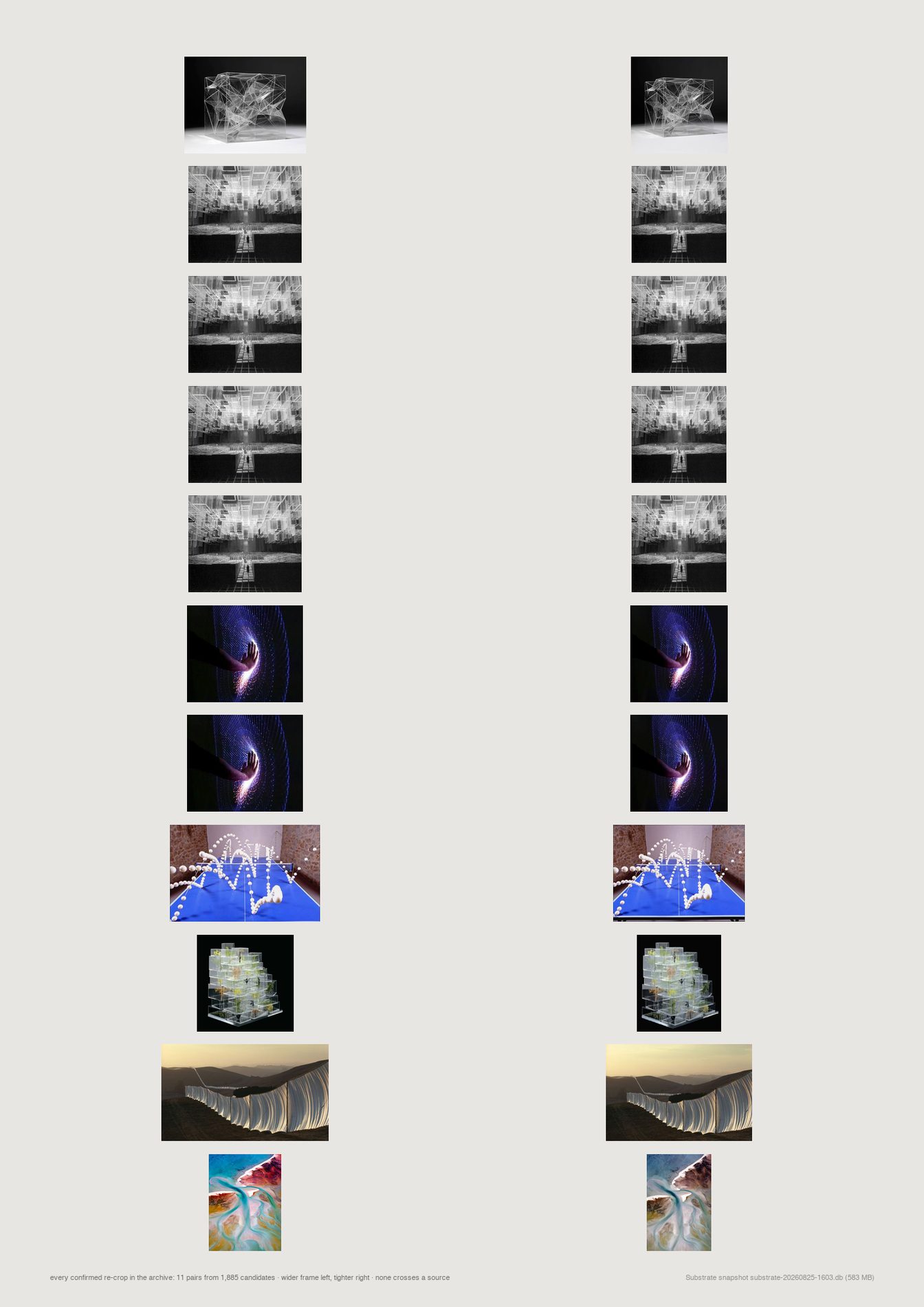
The brief asks for saved-against-source: retrieve the original, align it, show what was left outside. That comparison is not available in this archive, and the failure is specific enough to be worth recording.
Every duplicate family was searched for members whose aspect differs by more than 10%: 1,885 candidate pairs.
Those are candidates and not crops — the perceptual hash resizes to a fixed 8×8 grid, so it is aspect-blind and matches structurally similar pictures freely. Confirming each pair against its two CLIP image embeddings, which are not aspect-blind: 21 pairs at CLIP ≥ 0.85, 11 at ≥ 0.90, 8 at ≥ 0.95.
Eleven. In 26,214 references there are eleven cases of the same image saved twice at two different framings, and not one crosses from one platform to another — all eleven are pinterest to pinterest.
That is a result rather than a failed run. The studio does not re-crop what it already has, and the archive holds no before-and-after pairs to argue from. The sheet draws all eleven at once, which is the entire population and fits on one page.
A null with a population of eleven is more useful than the sheet the brief asked for would have been, because it says the question cannot be answered here rather than answering it on eleven cases. Ten of the eleven keep the same subject label on both sides.
Read the 26,214 alongside the d19 sheets: d16_crop and d19_frames both call d19_formats.load(), so this is one population reported twice and a change to it moves both. See the note under the frames sheets.
What would make this wrong. The candidate list comes from perceptual-hash families, so a re-crop tight enough to change the structure of the picture would never enter the 1,885 and could not be confirmed. Eleven is a floor, not a count — but the platform result holds regardless of the floor, because the mechanism that would produce cross-platform pairs is a person re-saving the same picture from two places, and none of the 1,885 candidates does that either.
python3 src/publish.py d16-recrops
# python3 src/viz/d16_crop.py --mode pairs --page a3 --dpi 120
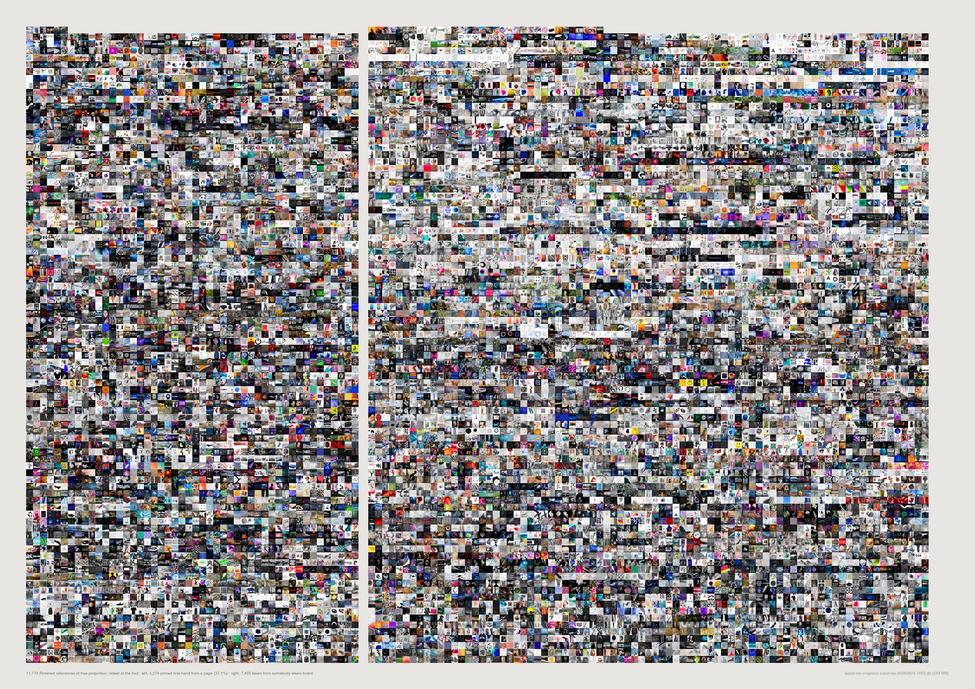
Pinterest's export carries parentPinId on every pin — the pin it was repinned from. Of the 11,902 pins live in Substrate and surviving the pool:
taken from somebody else's board 7,407 (62.2%) · pinned first-hand from the web 4,389 (36.9%) · re-saved from the studio's own pin 106 (0.9%).
A pin with no parent was saved from a page.
A pin with a parent was saved from another pinner's board — already collected, already framed, already captioned by somebody else, and the studio took the whole package.
And it moves, in one direction, across fourteen years. 2012: 71.3% first-hand (on 195 pins, so read it as a direction). 2016: 45.0%. 2018: 32.3%. 2023: 21.3%. 2025: 20.6%. 2026: 19.6%.
Where the two kinds of pin point is a second, independent signal that they are different acts. Reached first-hand: vimeo 386, instagram 225, youtube 193, google 157, behance 151. Inherited from other boards: behance 283, flickr 236, instagram 144, designboom 101, vimeo 97, archdaily 97, dezeen 81. What the studio found itself is moving image and portfolios. What it inherited is architecture and design blogs.
Project boards, the numbered ones opened for a live job, are more second-hand than the taste boards: 30.1% first-hand over 5,226 against 42.2% over 6,676. Under a brief the studio takes what somebody else has already gathered.
Aesthetic filter off. This is a sheet about the archive's own provenance, and a screenshot has a parent pin like anything else. Filtering to reference material would answer a different question. What the pool does change here is the 106.
1,089 pins in the export name another of the studio's pins as their parent. 106 are live — and all 106 were in dedupe.redundant(). Not most. All. A picture deliberately saved a second time was, to every measurement in this repo, a duplicate to be dropped, and the third category of provenance was empty in every deduplicated analysis including this one. pool.protected() puts them back: 106 dropped by the raw duplicate filter, 0 dropped by the pool.
Unlike the crop sheet, these two are drawn at true proportion — the first-hand field is 37.1% of the ink because it is 37.1% of the archive. Inside each field images run in date order, so the drift toward second-hand is visible as the fields change density up the page.
What would make this wrong. parentPinId records the pin a repin was made from, not the human act — a pin with no parent could have been saved with the browser button from a page, which is what “first-hand” is meant to mean, or created by an upload or a paste. And createdAt is the pin's date, which for a repin is the date the studio took it and not the date the picture entered the world. This covers Pinterest only; the other live references have no equivalent field, so nothing here is a claim about the archive as a whole.
python3 src/publish.py d17-provenance
# python3 src/viz/d17_biography.py --mode provenance --page a2l --dpi 150
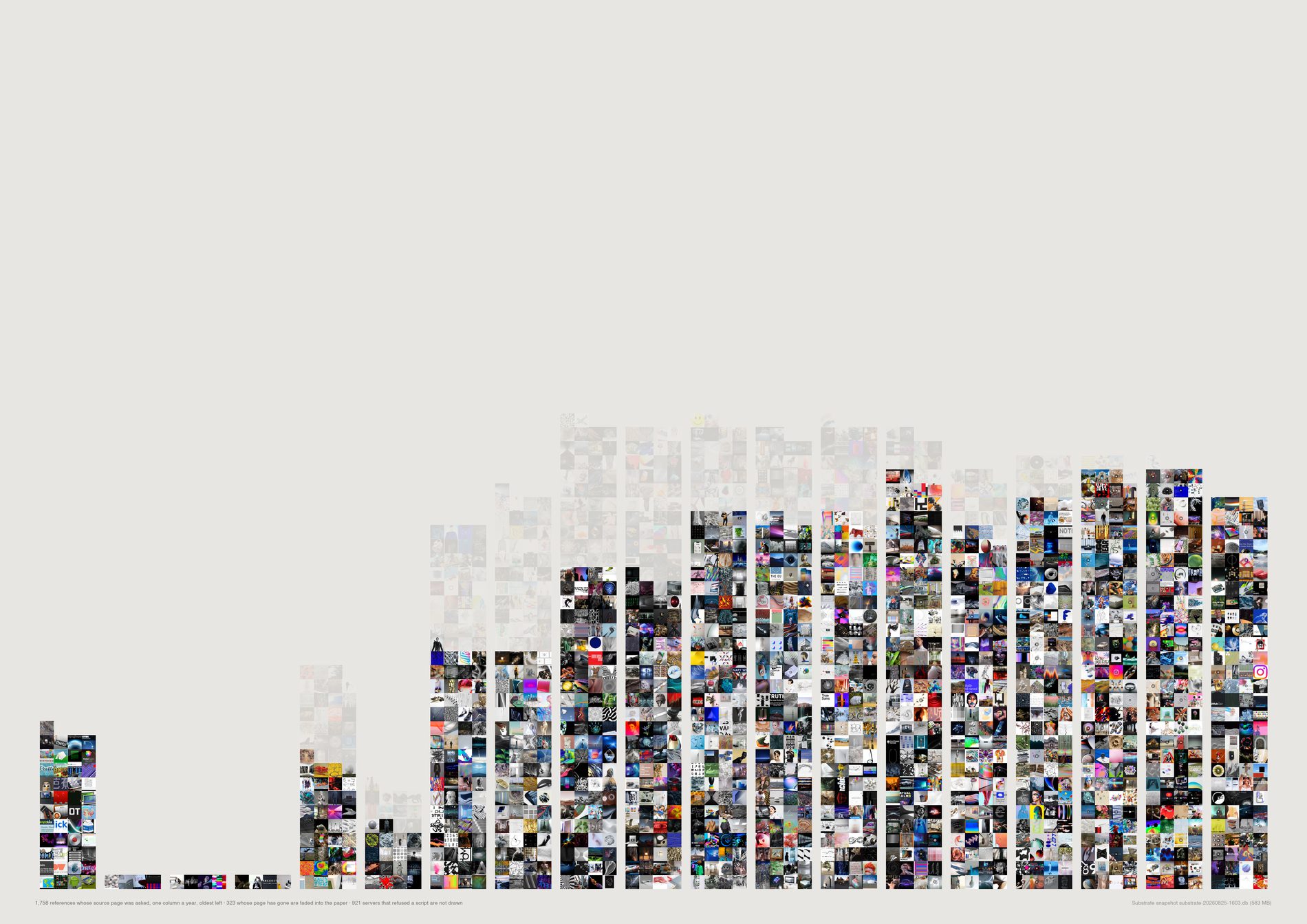
Of the references drawn here, 323 point at a page that is gone or a host that no longer answers — 18.4%. Split by the year the material was filed:
2012: 41.3% gone, over 63 references.
2015: 39.8% over 113. 2018: 19.4% over 134. 2021: 9.2% over 130. 2024: 3.3% over 123. 2026: 0.0% over 112.
Read against the survival side of the same check — the Pinterest subset of the link sample, 1,436 links, where the destinations are a genuinely diverse web, and slightly larger per year than the drawn columns because it does not require a cached picture: 2012 54.1% still answering over 63 links, 2015 59.6% over 123, 2018 78.5% over 139, 2021 88.1% over 110, 2024 90.4% over 59, 2026 100% over 11.
This is the argument for owning your own data, measured rather than asserted. Substrate holds the picture. The page it was taken from, for two in five of the 2012 links, does not exist at that address any more. A studio that had kept only the link would have lost two fifths of its 2012 research and all of the context around it.
A stratified survival check is only as good as its strata. d17_linkcheck.py takes up to 150 links per calendar year, 2008–2026, seed 7, from live references with a public http(s) URL, minus the duplicate filter and minus private hosts. Every year with enough material contributes exactly 150, so the sample is deliberately not proportional to the archive — it is built to make thin early years comparable with thick recent ones. 2,766 links checked, HEAD then a ranged GET, four outcomes kept apart.
refused — 401, 403, 429 — is a live server declining a script, not a dead page, so it is counted separately and left out of every survival rate. It is 33.3% of the whole sample, and 92.2% of CreativeApplications' 880 links. On the full sample the early years would be a measurement of one publisher's rate limiter, which is why the survival curve is quoted on the Pinterest subset (1,436 links, 68.6% still answering).
After refusals and the requirement of a cached picture, 2009, 2010 and 2011 fall to four references each and 2008 to 45. Those columns are on the sheet at their real size and they carry no information; the curve should be read from 2012 forward. This is the cost of a publisher-dominated early archive, and it is visible rather than smoothed.
What would make this wrong. A soft 404 — a dead article redirected to a live homepage — is not detected and counts as alive, so every survival figure here is an upper bound and every decay figure a floor. The check also ran once, from one network, on one day; a site down for an afternoon reads as gone. And the sample is of URLs the archive recorded, which for Instagram (391 links, 98.7% still answering) means a platform permalink rather than a page anyone published.
python3 src/publish.py d17-decay
# python3 src/viz/d17_biography.py --mode decay --page a2l --dpi 150
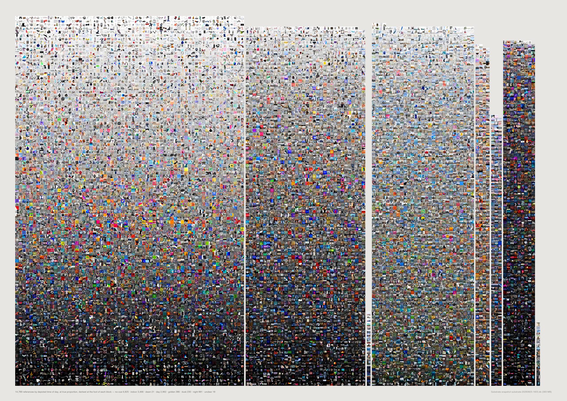
16,017 references, asked what time of day they depict: no-cue 7,871 (49.1%) · indoor 3,504 (21.9%) · day 3,043 (19.0%) · night 921 (5.8%) · golden 397 (2.5%) · dusk 236 (1.5%) · dawn 23 (0.1%).
71.0% of what this studio has collected depicts no hour of the day. Only 4,620 references, 28.8%, carry a readable outdoor time.
Season is thinner still: 90.8% is seasonless and the four seasons together account for 1,233 images.
Dusk beats dawn ten to one — 236 against 23 — a real asymmetry and not an artefact of anything the model was asked.
And the light is not the sun. Artificial 48.1%, sun 15.2%, none 14.9%, screen 8.2%, sky 6.8%. The archive is lit by lamps, LEDs and screens: a record of interiors, studios, galleries and rendered space.
Asked instead about the age of the thing shown: contemporary 66.1%, timeless 28.2%, c20 3.0%, future 1.7%, historic 0.8%, ancient 0.2%, prehistoric 0.2%. 1.1% depicts anything made before about 1900. The hoped-for story of an archive in conversation across radically different historical times is not what the pictures show.
This script was still calling dedupe.redundant() directly. The decision is not close: the headline is what share depicts no hour, and a link card, a screenshot and a page of typography are all no-cue by construction — pictures of nothing at any time. Counting them counts the answer into the question. Default pool, 1,716 references dropped, 17,733 to 16,017. The finding survives and softens: no-cue 52.0% to 49.1%, no-hour 72.5% to 71.0%. The clearest evidence the filter did the right thing is the lighting column, where none falls from 19.6% to 14.9% — the dropped material was disproportionately the material lit by nothing.
A model asked “is this night?” will answer, so the answers are checked against something that was not the model. measured.json holds brightness_med for every one of these images, measured off the pixels months before this pass existed: night 0.172 · dusk 0.339 · indoor 0.416 · golden 0.474 · day 0.514 · dawn 0.533 · no-cue 0.557, against 0.484 for the whole set. Monotone from night through dusk and golden to day, on an independent measurement, over 921 and 236 and 397 and 3,043 images.
One band across the page, each segment one column per cell width, so a segment's area is its count and nothing is scaled anywhere. Dawn is one partial column, 23 cells in a field of 16,017, because that is what dawn is here. Inside each segment images run by measured brightness, so the validity check is not only printed but visible: the night block reads dark and the day block reads light, and nothing arranged them that way except two independent measurements agreeing.
What would make this wrong. Brightness agreeing with the label does not prove the label — a dark studio shot and a night street both read dark. The check rules out the failure mode where the model answers from the prompt rather than the image; it does not certify any individual record. Dawn at 0.533 on 23 images is the one bin too small to trust, and it is drawn at that size, which is the honest way to show it.
python3 src/publish.py d18-daytime
# python3 src/viz/d18_daylight.py --mode daytime --page a2l --dpi 150
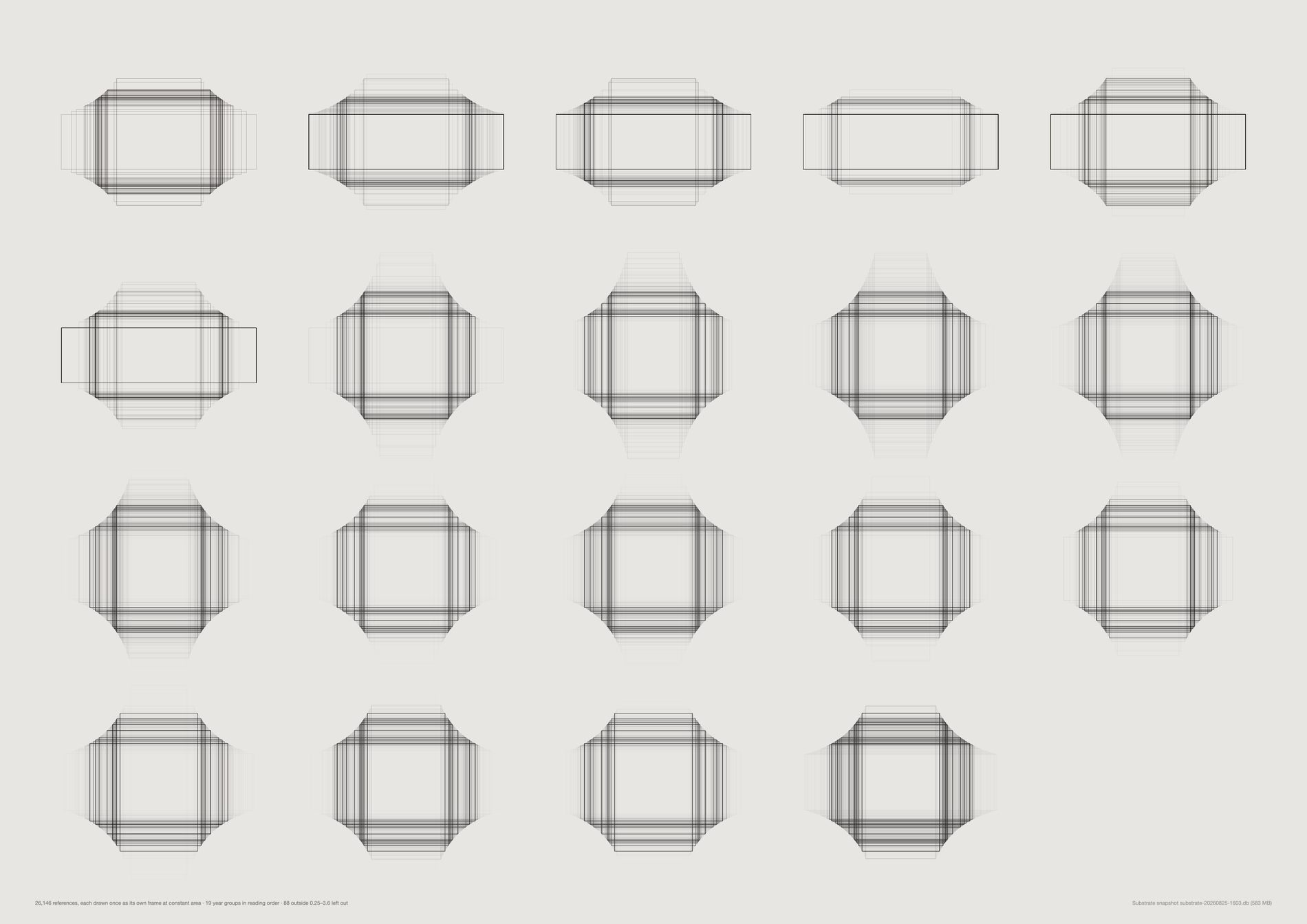
The shape of this archive changes completely across nineteen years:
2011 — ultrawide 74.3%, square 0.4%, tall 0.0% (245 references)
2015 — ultrawide 0.8%, square 9.6%, tall 31.9% (492)
2021 — ultrawide 0.8%, square 23.8%, tall 19.8% (1,097)
Read as a story about taste that is dramatic: the studio abandons the panorama, discovers the portrait, then the square.
It is not a story about taste, and the source column explains all of it. See the sheet below.
The modal shape per year is the plainest version of it: ultrawide in 2009, 2011 and 2012; wide in 2010, 2013, 2014, 2016, 2017, 2019–2022 and 2026; tall in 2015, 2018 and 2023–2025. Those are not aesthetic eras. They are which pipe the intake ran through.
Every frame is drawn at the same area, so an ultrawide and a portrait carry the same ink and shape is the only difference the eye can see. Scaling to constant height would make wide images look important and tall ones look small, which is a claim about attention this data cannot support.
Outlines pile up at a year's modal shape and fade at its spread, at an opacity that falls with the count so a thin year and a thick year stay comparably legible. It is the same construction as an exposure stack, and it is the only one of the three forms that makes nineteen years comparable at a glance.
references_.created_at is the pin's own date on Pinterest and the article's date on CreativeApplications. For a blog archive imported in bulk that means the early years are the blog's publishing history rather than anyone's browsing history — which is exactly why the ultrawide era looks so clean.
What would make this wrong. Resolution is deliberately absent: the cached files are Pinterest derivatives — 9,333 of them exactly 282px wide — so a resolution axis here would describe this repo's downloader. Aspect survives the derivative and was checked rather than assumed, against Pinterest's native dimensions on 14,516 pins, matching to a median relative error of 0.00043 with 100% inside 2%.
python3 src/publish.py d19-windows-year
# python3 src/viz/d19_frames.py --by year --page a2l --dpi 150
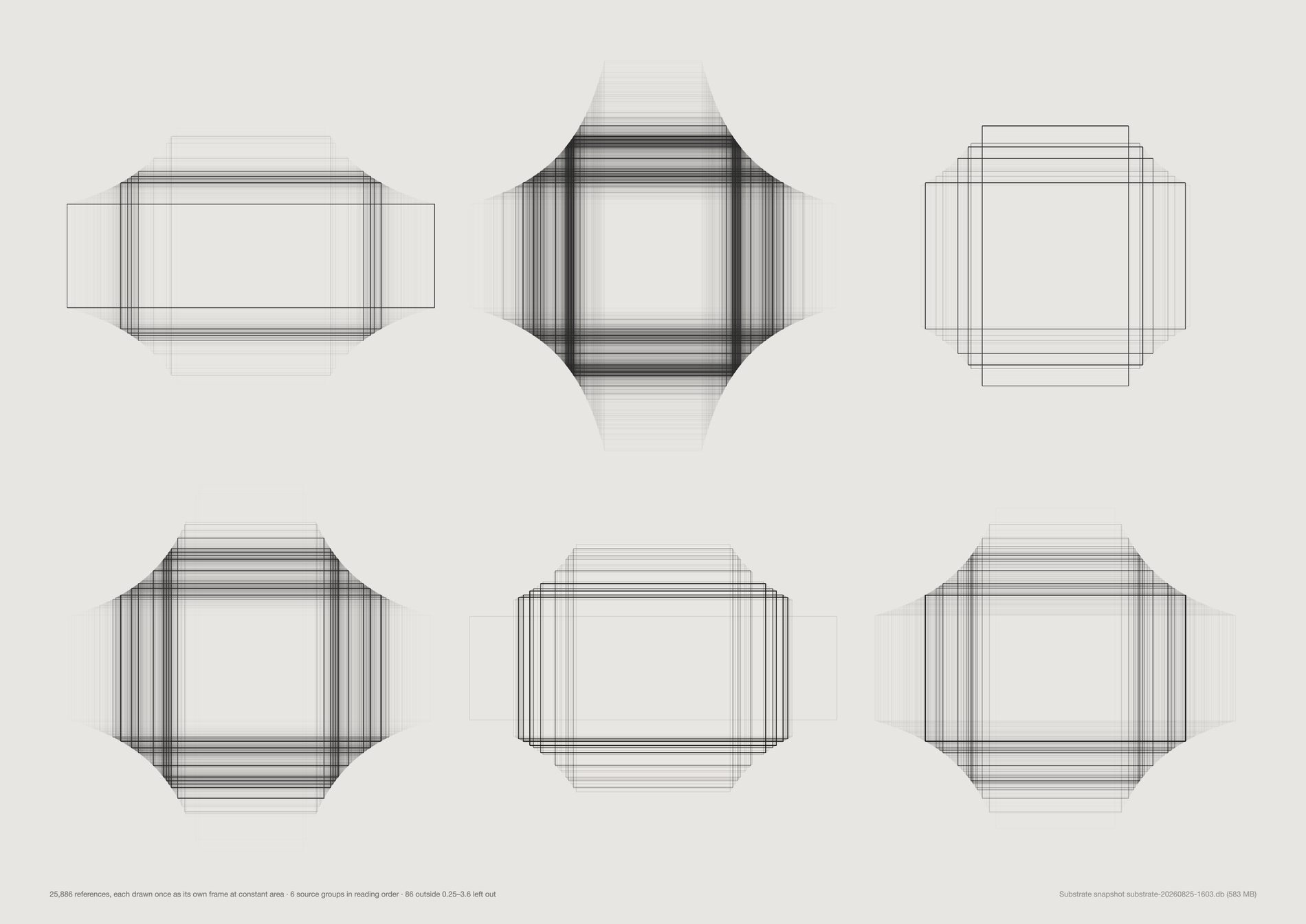
creativeapplications — wide 56.9% + ultrawide 32.1%, so 89.0% landscape or wider. Its WordPress theme crops every post header to 3.545:1, and 648 references sit on that exact ratio to the pixel.
pinterest — tall 27.7% + portrait 18.9%, 46.6% upright. A portrait feed.
instagram — square 49.8%. Square by decree until 2015 and square by habit after.
basecamp is wide 38.8% and manual 63.2%, which is what files dragged into a project thread look like.
So the years the archive is ultrawide are the years its intake ran through a blog, and the years it is square are the years its intake ran through a phone. The guardrail — avoid claiming a platform from dimensions alone — is answered by never having to: every reference carries a recorded source, so this sheet shows the attribution directly rather than inferring it from the shape.
Aesthetic filter off. This is format archaeology and a screenshot has a shape like anything else. Filtering down to reference material would remove exactly the rows that explain the shape — the CreativeApplications header crop, the Pinterest derivative widths — and turn a finding about publishing formats into one about taste. What the pool does change is that the studio's 106 deliberate re-saves are no longer discarded as duplicates: 26,214 references before, 26,214 after.
d19_frames.py and d16_crop.py both call d19_formats.load(), deliberately, because both turn on the same question — where did this rectangle's proportions come from — and neither should be allowed to answer it differently. The 26,214 and the 23.4% hand-cut figure are the same numbers on both sheets, and a change to d19_formats moves the crop sheet too. They are coupled by design; the coupling is stated here rather than discovered later.
1:1 2,798 · 16:9 1,888 · 2:3 1,527 · 3:2 1,505 · 4:5 977 · 4:3 933 · 3:4 833 · 9:16 787. Nobody arrives at 1.7778 by eye.
What would make this wrong. Five groups cover 17,965 of 26,214 — the small sources are not drawn, and github, linkedin and upload are tens of references each. Source is a recorded field rather than an inference, which is this sheet's strength, and it records where the reference entered Substrate, not where the picture was made.
python3 src/publish.py d19-windows-source
# python3 src/viz/d19_frames.py --by source --page a3l --dpi 150
The brief's literal request, and the texture change is visible with no grouping at all: the wide band across the top is 2008–2013, and the field turns upright and then square as it descends.
It is the same population as the two window sheets — 26,214 references, aesthetic filter off — drawn once each rather than stacked, so nothing is hidden behind anything.
An outline at constant area carries exactly one variable. Put the photographs back in and the eye reads subject matter, which is a different sheet and is the one below.
The date is the material's, not the finding's. The clean band at the top is a blog's publishing history arriving in bulk.
What would make this wrong. This is a visual study and makes no claim on its own. Every measured statement about it lives on the two window sheets, which is where the source attribution is.
python3 src/publish.py d19-wall
# python3 src/viz/d19_frames.py --mode wall --page a2l --dpi 150
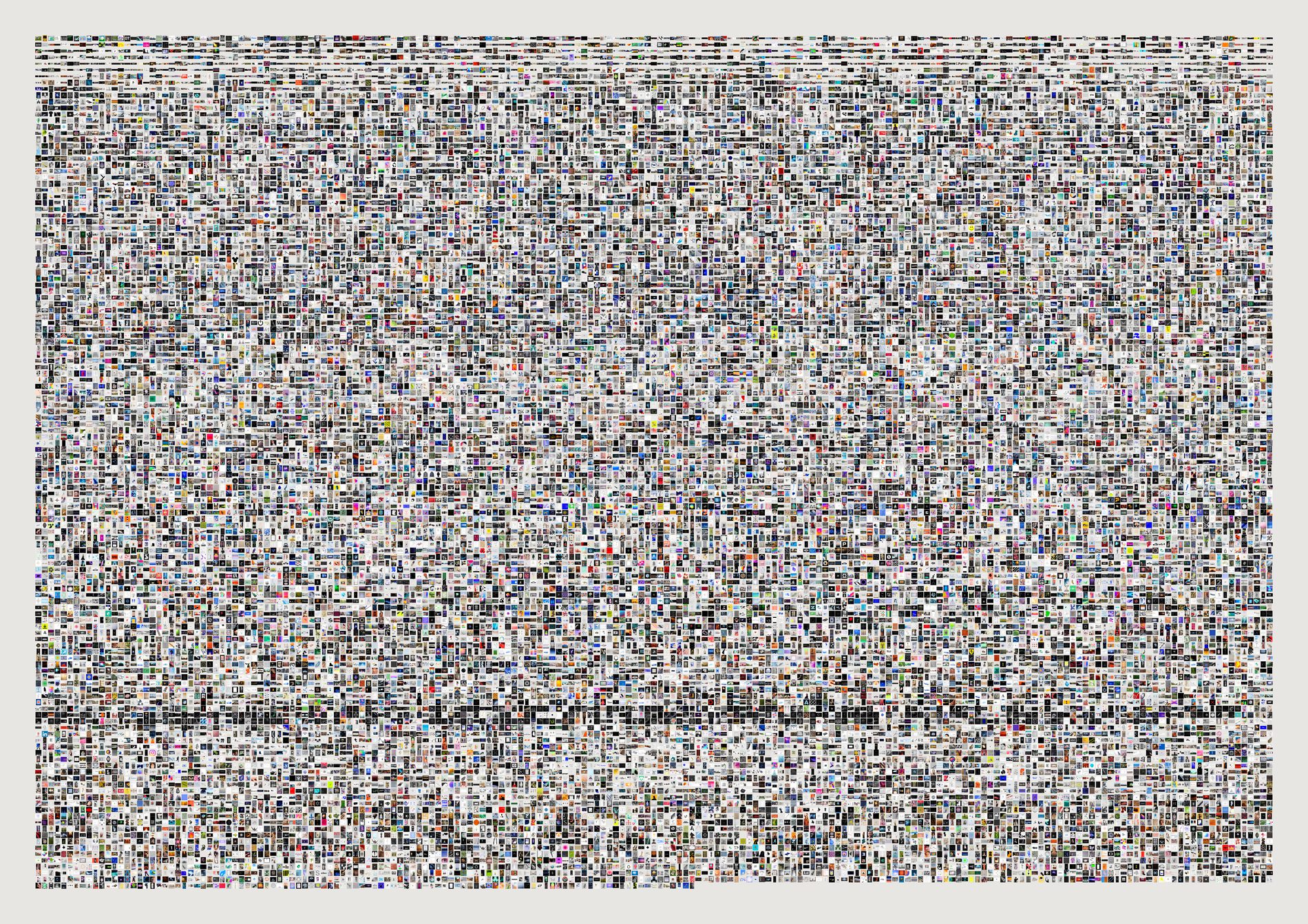
The only sheet in this repo that does not square-crop, and it is that way on purpose: squaring the cells would destroy the one variable the sheet is about.
All 26,214 cells filled — no cache misses, no skipped frames. Read beside the empty wall above, it is the same argument with the subject matter switched back on: the shape change is still legible underneath the pictures, which is the point.
Unlike the other three, this mode composites directly into a raster at 200dpi rather than emitting an SVG. Eighteen thousand embedded images in one vector file is not a printable object.
Where a cell's picture does not fill its allotted square, the paper shows. That negative space is the aspect distribution, drawn as an absence.
What would make this wrong. Visual study, no claim. At this scale an individual cell is about eight pixels on the published JPEG and the sheet is honest only as a texture — the print file is 4,677px wide and is the one worth looking at closely.
python3 src/publish.py d19-wall-filled
# python3 src/viz/d19_frames.py --mode filled --page a2l --dpi 200
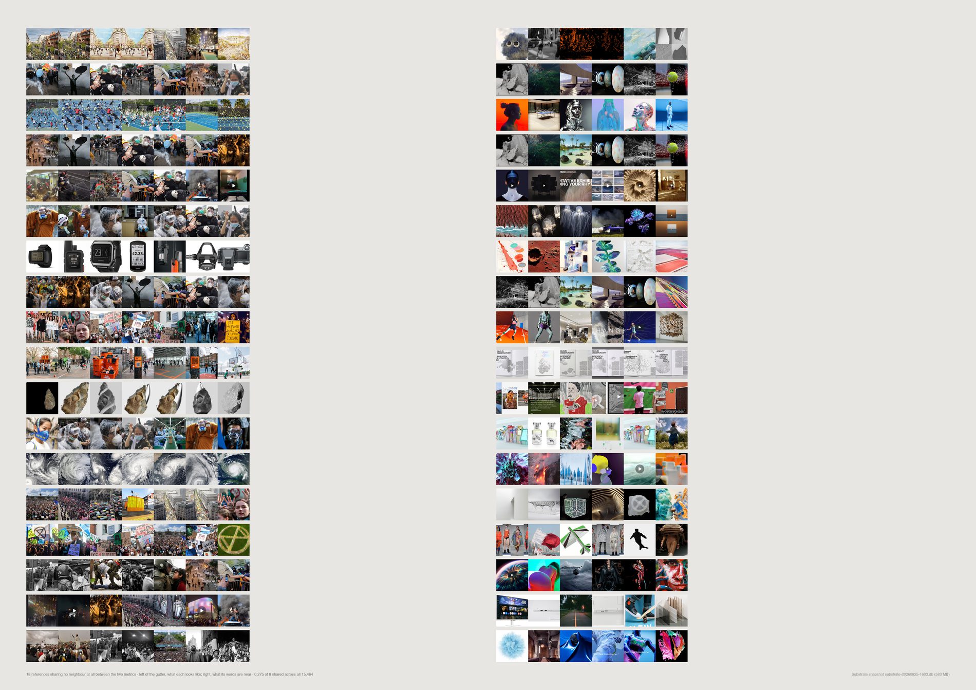
The archive carries two independent descriptions of every reference, built for different purposes by different models. CLIP image vectors — 512-dimension, computed in this repo from the cached picture; “similar” means looks like.
voyage-3 text vectors — 1024-dimension, built inside Substrate from each reference's title and scraped description; “similar” means is described like.
Over the 16,569 references carrying both, comparing the top eight neighbours under each metric:
mean overlap@8: 0.253 of 8 · share nothing at all: 13,724 (82.8%) · share exactly one: 1,989 (12.0%) · share four or more: 116 (0.7%)
Five references in six have a visual neighbourhood and a linguistic neighbourhood with no member in common. Substrate's own search runs on the text vectors. This sheet is what that search is not showing you.
Both halves of every row are real pictures, which is the only way to make the point: the left half looks like the anchor, the right half is about the same words, and they are different sets of things.
They were never mixed. Two matrices, two metrics, computed independently and never averaged into a single “similarity”: a 16,569 × 16,569 cosine pass under each, top-8 taken from each, and the only quantity compared is set overlap — how many of one list appear in the other. That is a measure with no free parameters and no shared axis, so neither space can flatter or contaminate the other. The guardrail is that neither side is the truth: this is a comparison between two models, not between a model and a person.
Default pool. The temptation was to keep everything and call this archive structure — but a link card is the one object where text-image disagreement is true by construction and means nothing, since its picture is a publisher's thumbnail and its text is a headline. Filtered, the finding is about reference material. And it barely moves: overlap@8 is 0.253 either way, and share-nothing goes 83.0% to 82.8% over 16,569 references instead of 18,272. So the disjointness is a property of the two embedding spaces, not an artefact of link cards.
Direction 17 measured that 62.2% of the Pinterest archive was taken from someone else's board, and the description usually comes with the pin. So a good deal of the “linguistic neighbourhood” is other people's language about this studio's pictures. That does not weaken the disjointness; it changes what it is a finding about.
What would make this wrong. Overlap@8 is sensitive to k, though not enough to change the story — the disjointness holds because the two spaces are built from different inputs, not because eight is a small number. A reference whose description is empty still gets a text vector from its title alone, and about 2,265 references have no description at all, so those are noisier on the linguistic side by construction.
python3 src/publish.py d20-neighbourhoods
# python3 src/viz/d20_naming.py --mode neighbours --page a2l --dpi 200
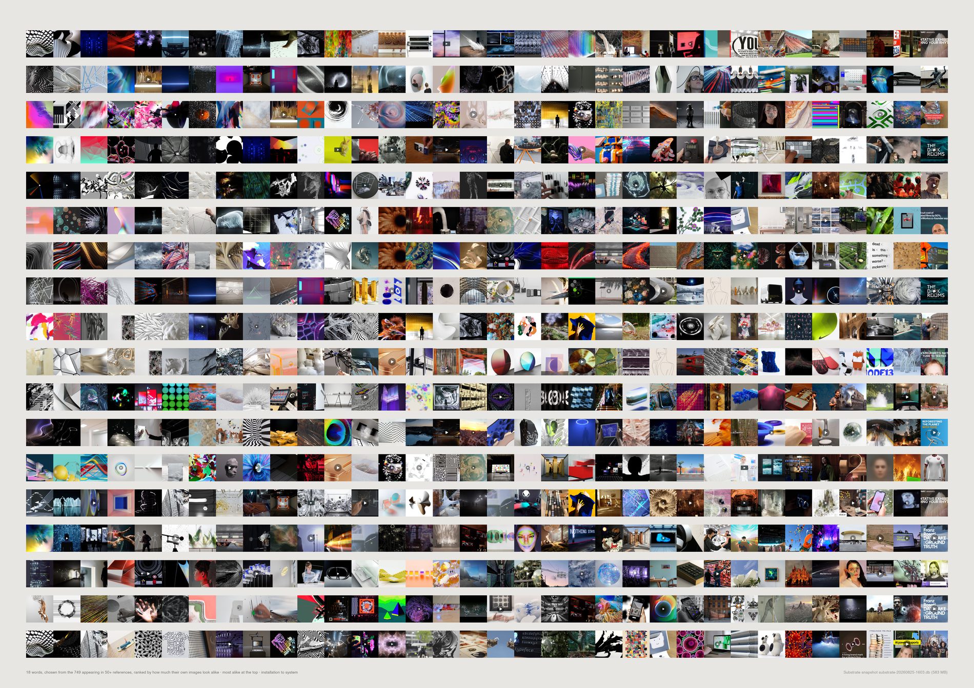
For every word appearing in the title or description of fifty or more references, the mean cosine of that set to its own CLIP centroid — how much the images sharing a word look alike — against a size-matched random baseline.
834 words qualify.
Most visually coherent: installation 836 refs z +15.8 · light 653 z +13.6 · generativeart 119 z +11.2 · abstract 315 z +10.4 · touchdesigner 115 z +9.5 · glass 181 z +9.2 · sculpture 319 z +8.1.
At or below baseline, and these are the studio's own vocabulary: system 228 z +0.3 · technology 282 z +0.2 · human 211 z +0.7 · experience 299 z +0.8 · spatial 61 z +1.0 · brand 150 z −1.9 · future 258 z −2.5.
It is not abstraction that separates them. abstract is among the most visually coherent words in the archive at z +10.4. The dividing line is whether the word names something an eye can check. Light is a thing you can photograph. System is a thing you can only claim.
Of the five words the brief nominated — organic, intelligent, spatial, alive, system — intelligent and alive appear in fewer than fifty references and cannot be measured at all, spatial and system sit at baseline, and only organic (81 refs, z +3.3) shows anything.
The least coherent words are have (494, z −8.0), friends (102, −7.2), even (113, −7.1), now (380, −7.1), today (164, −7.0), world (565, −6.8) — caption filler and function words, exactly the vocabulary that should carry no visual signal, and does not. screenshot at 126 refs and z −5.6 is a word about the file rather than the picture.
Under the old duplicate-only population, system scored z −2.7 and spatial −1.4 — measurably below a random handful of the archive. Under the pool they are z +0.3 and +1.0. The honest claim is now “at baseline” rather than “below”, which is weaker, and it is the number the sheet is drawn from. The rank order and the argument survive; the sharpest version of the sentence does not.
No number is drawn anywhere on the sheet. A coherent word reads as a run of one kind of picture and an incoherent word reads as noise, and the row is the evidence for its own position. Rows run most coherent at the top to least at the foot.
What would make this wrong. Word sets are matched on raw substring tokens with a short stoplist, so light the noun and light the adjective are the same set, and homonyms are never separated. Coherence rewards a set that is tight anywhere in the space — it is not a quality score and must never be read as one. A low score is not a criticism of a word: system failing to predict a picture is exactly what you would expect of a word naming an intention rather than an appearance, and that difference is the argument, not anyone being wrong.
python3 src/publish.py d20-words
# python3 src/viz/d20_naming.py --mode words --page a2l --dpi 150
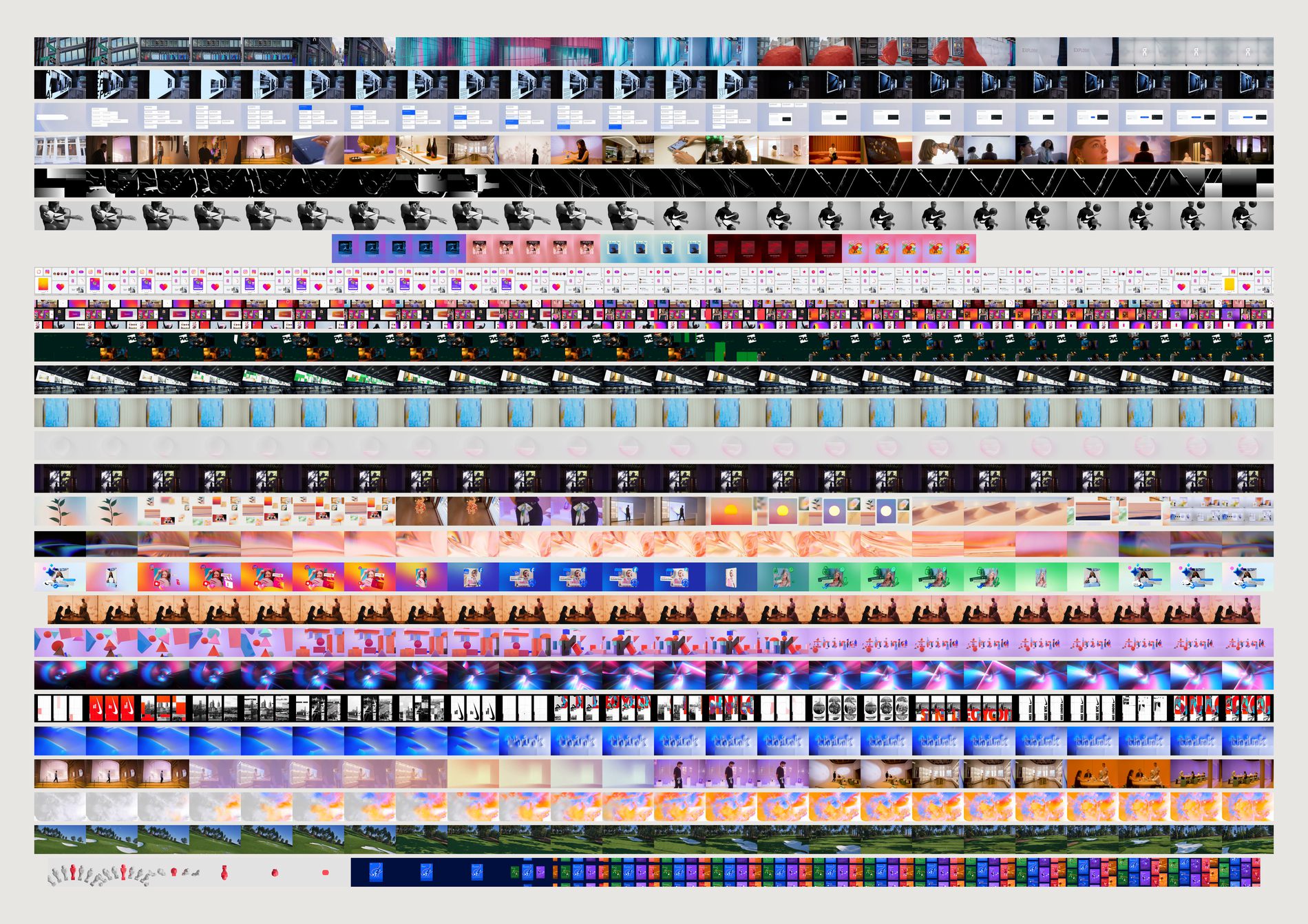
The video work is the only material in the archive that can carry a verb. The studio's own brief argues that FIELD's signature is a set of verbs — dissolve, refract, fragment, swarm, reveal — and a verb is temporal. CLIP on a single frame cannot tell dissolve from refract: same pixels, different moment. 418 of Canopy's published media are .mp4, across 107 of 176 published works, and until these were downloaded none of it was on disk.
The two sheets after this one are reductions. A reduction is only trustworthy next to the thing it reduced, so this is the one that lets you check them: same pieces, same order, whole pictures.
418 published mp4s; 416 cached (two failed — one asset 404ing under two work records); 132.5 minutes of footage; 24 evenly spaced frames from each, 9,984 frames in all. A sheet drops anything under 1.5 seconds, which leaves 414: the two dropped are 1.0s and 1.24s. Pieces run 1.8 seconds to 453.9 seconds, median 12.5.
In arbitrary order this is a contact sheet. Sorted by edge slope it runs from the pieces that lose edges over their length to the pieces that gain them, which is as close as measurement gets to sorting dissolve from assemble. Of the 414: 148 lose structure, 163 gain it, 103 sit flat inside ±0.005. When more pieces qualify than the page holds, the sheet walks evenly down the whole sorted order rather than taking one end of it and implying it is the range.
These come from Canopy's published media, not from the reference archive, so the evidence pool in src/pool.py does not apply and never filtered them. What they are instead is curated by the client: these are the pieces FIELD chose to show and someone approved. And Cloudinary re-encoded them at w_480,q_auto:eco, so fine grain is gone and edge density reads systematically low — consistently across all 416, so comparisons hold and absolute values do not travel.
What would make this wrong. The rows are not on a common time axis. A four-second loop and a seven-minute film are both stretched to the same 24 cells, so cell position compares within a row and never between two. That is deliberate — a real time axis would reduce most of the sheet to a sliver — but it means nothing here measures duration. And 24 samples is a coarse net. The longest piece in the set runs 453.9 seconds and is read once every 19 seconds; anything that happens between two samples did not happen as far as this sheet is concerned. Frames are letterboxed rather than cropped, so a square loop draws a thinner ribbon than a 16:9 film: 50 distinct aspect ratios across the 416, of which 301 are 16:9. That raggedness is real information about the formats FIELD publishes in.
python3 src/viz/filmstrip.py --sort structure --dpi 300
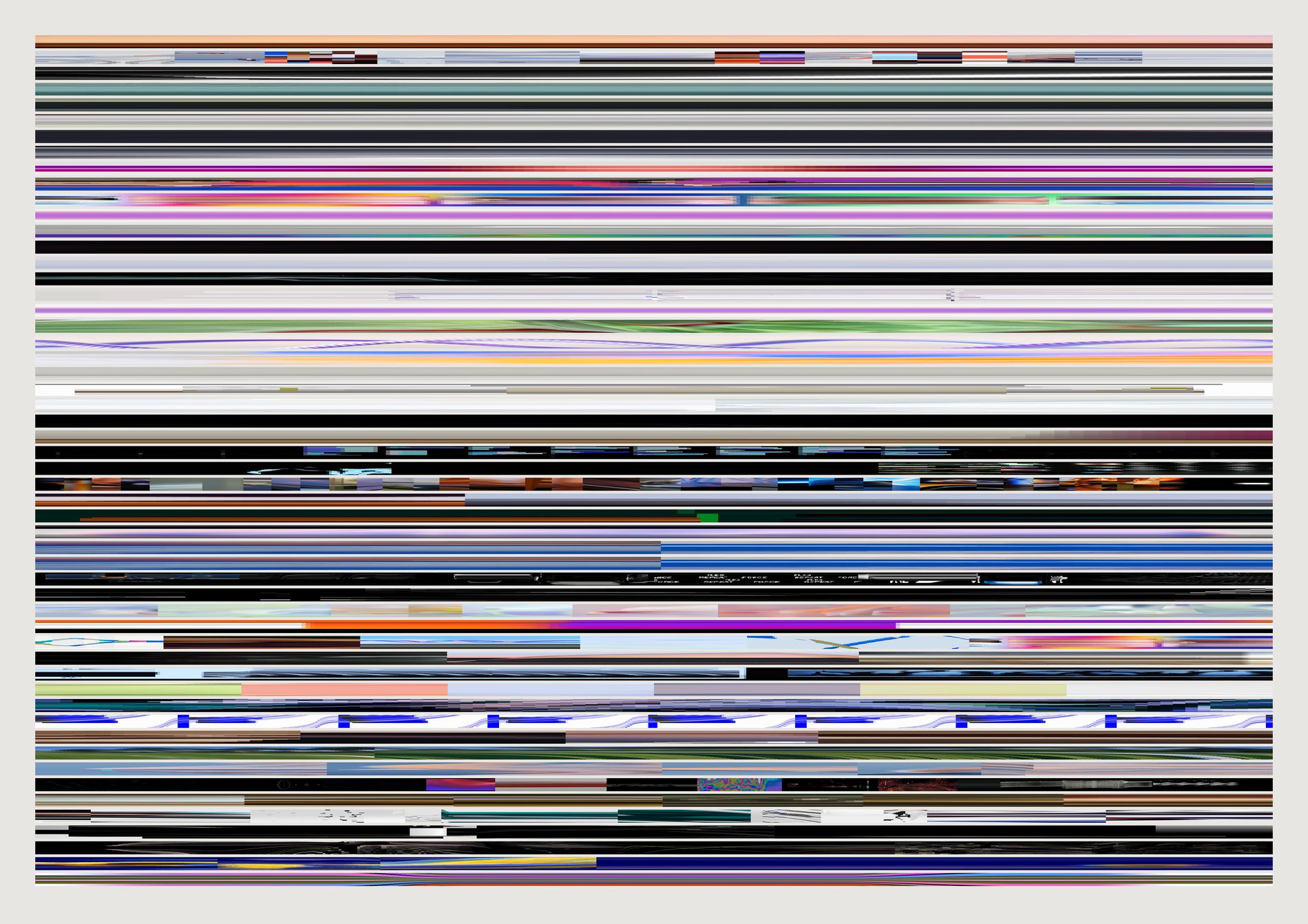
217 of the 414 pieces show no cut at all, and the two most heavily edited show ten each. The published motion work is overwhelmingly continuous — things that move, dissolve and drift inside a held frame — rather than edited.
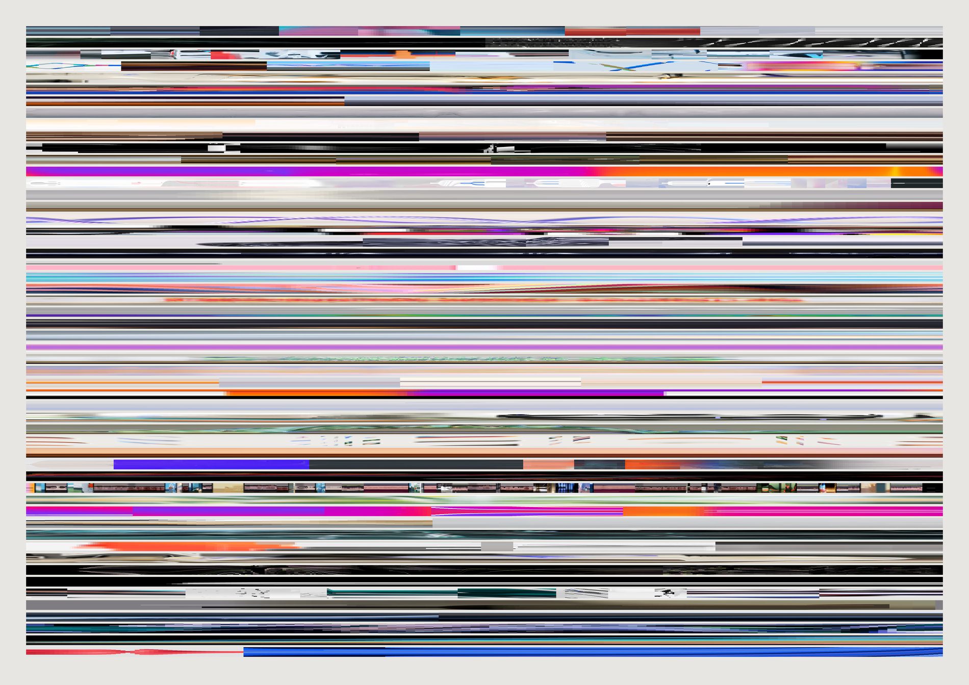
That is a claim about FIELD's house grammar that no still-image measurement could have made, and it is legible without a key: the flat fields at the top of the sheet are the pieces that hold, and the hard vertical stripes at the bottom are edits you can count.
The caveat travels with it. A cut is only a cut if it lands between two of the 24 samples the ordering was measured from. A fast cut back and forth reads as no cut at all, so 217 is zero cuts at this sampling and never zero cuts. The number to distrust is the low one.
A flat field is a piece that holds. Hard vertical stripes are cuts. A smooth horizontal gradient is a dissolve or a slow drift of palette. Wavering horizontal streaks are something moving through a held frame — a camera push, a swarm, a flow. None of that needs a legend and none of it needs playback, which is the whole reason the form survives print.
Worth separating, because the two halves of this sheet have different sampling. A band is built from real frames, 72 to 1,200 of them, capped at the video's own frame count so ffmpeg never duplicates its way to a smoother-looking piece. The order they are stacked in comes from the 24-frame measurement. So the picture is fine-grained and the ranking that arranges it is not, and a piece can be in slightly the wrong row while its own band is honest.
The sort is the piece. Ordered by cuts, the sheet separates continuous work from edited work. Ordered by structure it runs from pieces that lose edges to pieces that gain them. Same 54 bands drawn the same way both times: the only thing that changed is the question, and the eye finds the break point on its own in each.
What would make this wrong. The centre column is an arbitrary sample of the frame. A piece where everything happens at the left edge reads as a flat field here and is not one — a real failure mode, and the reason this sheet is only trustworthy read against the filmstrip above it. Columns are not seconds: a band spans the whole piece whatever its length, so stripe spacing compares within a band and never between two. And a short piece has fewer frames than the band has pixels, so its columns are stretched and its stripes are correspondingly fatter; the thinnest band here rests on 72 real frames against another's 1,200.
python3 src/viz/motion_signature.py --sort cuts --dpi 300 --columns
python3 src/viz/motion_signature.py --sort structure --dpi 300 --columns
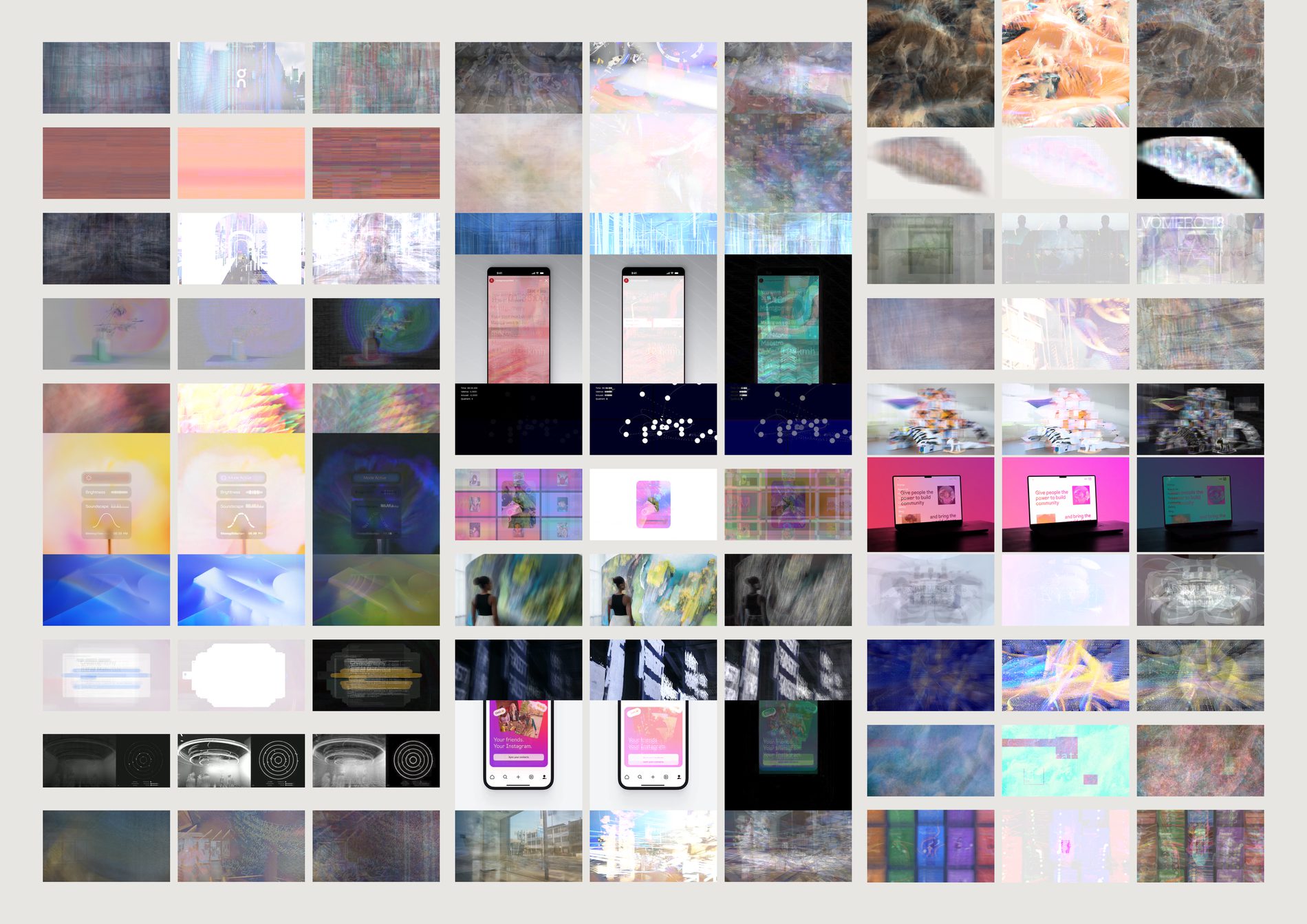
Difference is the mean absolute frame-to-frame change per pixel: black is where nothing moved, bright is where everything did. It separates a locked camera with action inside it from a piece where the whole frame travels, which is exactly the distinction a single frame cannot make and the one the verb question turns on. Read down the right-hand panel of each triptych and the studio's quiet work prints dark while the busy work prints as a lit rectangle.
Adding 24 frames and clipping at white was tried first. Re-measured on a fresh random 40 of the 414: the median piece clips every one of its pixels, and 38 of the 40 clip more than half. A literal sum of this corpus is a white rectangle 414 times over, and scaling it back down to fit recovers the mean image exactly, which is already panel one. So the middle panel is the brightest value each pixel reached — light accumulated the way a long exposure accumulates it. Calling it “sum” without this paragraph would be the kind of small lie that prints.
The difference panel uses a fixed linear gain and gamma, never a per-video normalisation. Normalising each piece to its own maximum would make every panel equally bright and destroy the only thing worth comparing across the sheet. The curve is there because the corpus has a 531:1 range in frame difference — 0.0006 to 0.3188 — and any linear exposure that keeps the busiest pieces off white leaves the median almost black. It is monotonic and identical for all 414, so it compresses the distance between ranks and not their sequence. A quiet piece is meant to print dark.
A hard cut lights the entire difference panel; so does a whip pan; so does a swarm filling the frame. The panel says the pixels changed and the filmstrip says why. Nothing on this sheet is a verb label, and the gap between a descriptor and a verb is exactly where a person has to do the interpreting.
What would make this wrong. All three panels are built from 24 evenly spaced samples, not from every frame, so the average is an average of a sample and the difference is a difference between samples that can be half a second or nineteen seconds apart depending on the piece. Raising the sample count costs time linearly; it does not change what any panel means, but it does make the smear smoother and the difference brighter. And a cut in a dark scene reads quieter than a cut in a bright one, because this measures absolute pixel change and not perceived change: two identical edits, one at night and one in daylight, print at different weights.
python3 src/viz/difference.py --sort structure --dpi 300
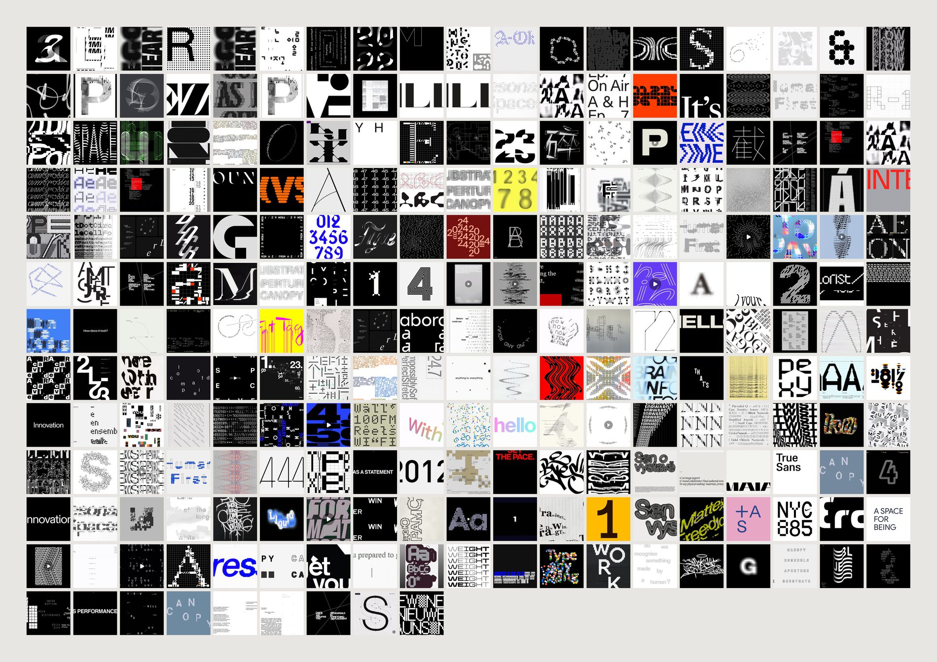
A vision model labelled 1,119 images in this archive made: typography. Dropping near-duplicates leaves 875.
Then the evidence pool's aesthetic filter runs and three survive.
That is not a bug, and it is the clearest worked example on this site of what the filter is for and what it costs. src/pool.py exists to answer what is FIELD's eye, and for that question a wall of type specimens is material the studio saved to read rather than material it saved because of how it looked — so removing it is right. For the question what typography does this archive hold, a three-image answer is useless. The filter is not a quality judgement, it is a scope judgement, and a sheet that quietly inherits the wrong scope answers a question nobody asked.
1,119 labelled → 875 after de-duplication → 3 after the aesthetic filter. The sheet draws the 240 most typical of the 875; four of those have no cached image, so 236 are on the page. Near-duplicates are dropped on both sides of the split — --unfiltered removes the aesthetic filter and nothing else.
Scored against the same centroid as everything else, the three survivors rank 37th, 180th and 665th of 875. So the filter is not keeping the most typographic typography and shedding the edge — it is keeping three images that happen to pass a test about taste, and their position inside the category is close to arbitrary. Dominant moods across the 236: modern, structured, clean, bold. Across the three: bold, modern, dynamic, urgent.
Cells run by cosine similarity to the CLIP centroid of the facet, most typical first, so you watch the category assemble and then dissolve at the edges. The labels are the model's, not FIELD's: it never saw the channel names, and it still reproduced the studio's own fourteen-year-old taxonomy. That makes the categories real. It does not make every individual label correct.
What would make this wrong. The population here is defined by a model's one-word answer to “how was this made”, and typography and graphic are not cleanly separable — a poster is both. A different labelling pass would draw a different 875. What survives that objection is the ratio: whatever the exact boundary, the aesthetic filter removes about 99% of whatever is inside it, and any sheet about the archive's type has to be run unfiltered or it is answering a different question.
python3 src/viz/facet.py --made typography --unfiltered --dpi 300
python3 src/viz/facet.py --made typography            # the three that survive the filter
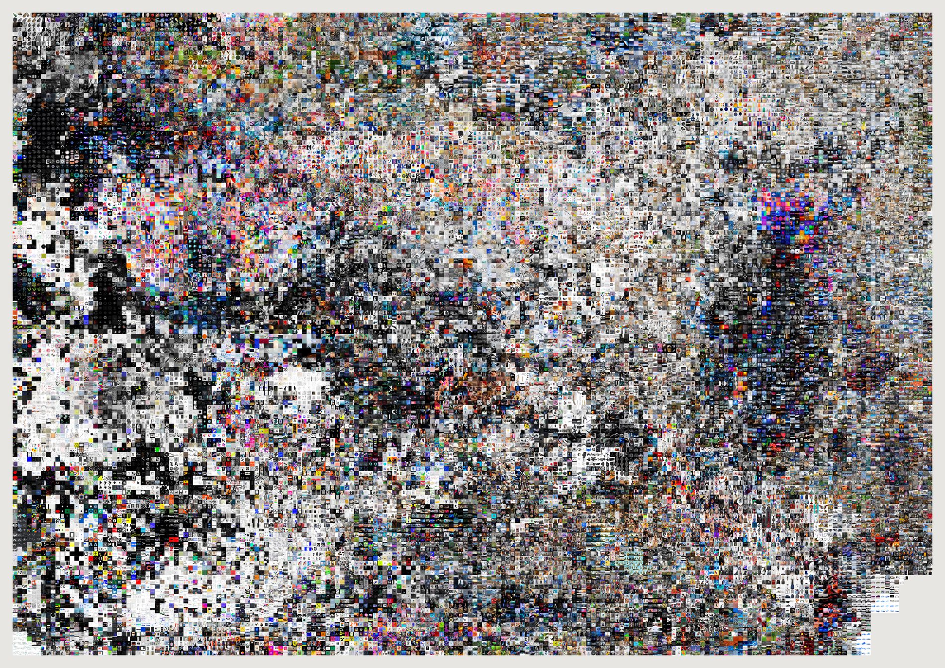
The published atlases all draw from the 21,491 references the evidence pool keeps, because the atlas is a sheet about taste and the screenshot continent that used to sit at one edge was a media-type artefact rather than a region of the eye. This is the same construction over the 26,214 the pool holds before that filter runs, and the extra 1,788 are not scattered evenly — they clump, and you can see the clump. It is the map of what the archive holds rather than the map of what the eye is, and the pair is the only honest way to show what the filter does to the shape of the thing.
By how they were made: 861 typography, 328 diagram, 265 photograph, 134 graphic, 116 render. By subject: 489 graphic, 403 typography, 345 data-visualisation, 139 interface. Type specimens, chart studies and interface captures — things the studio saved to read, not to look at.
This is a separate t-SNE run over a different set, not a zoom of the published atlas: 88 seconds over 26,214 points at perplexity 40, then a greedy snap onto a 162×113 lattice. Adding 1,788 points changes every neighbourhood a little, so regions here do not line up cell for cell with regions there.
The layout is not stable across runs unless the seed is fixed, and distance across the sheet is not proportional to distance in the embedding — snapping to a lattice deliberately distorts scale to remove gaps. Adjacency is meaningful; measured distance is not. Near-duplicates are dropped here exactly as they are in the filtered atlas.
What would make this wrong. Nothing here says the filter is a mistake — every sheet on this site that asks what FIELD's eye is should keep it, and this one would be the wrong sheet for that question. What it says is narrower: the filter removes about 10% of the archive and that 10% is a place, not a scatter. If a later pass moves the boundary, this sheet moves with it, so it is dated by its pool the way the corridor is.
python3 src/viz/atlas.py --unfiltered --max 30000 --page 1189x841 --dpi 200 --out atlas-dense
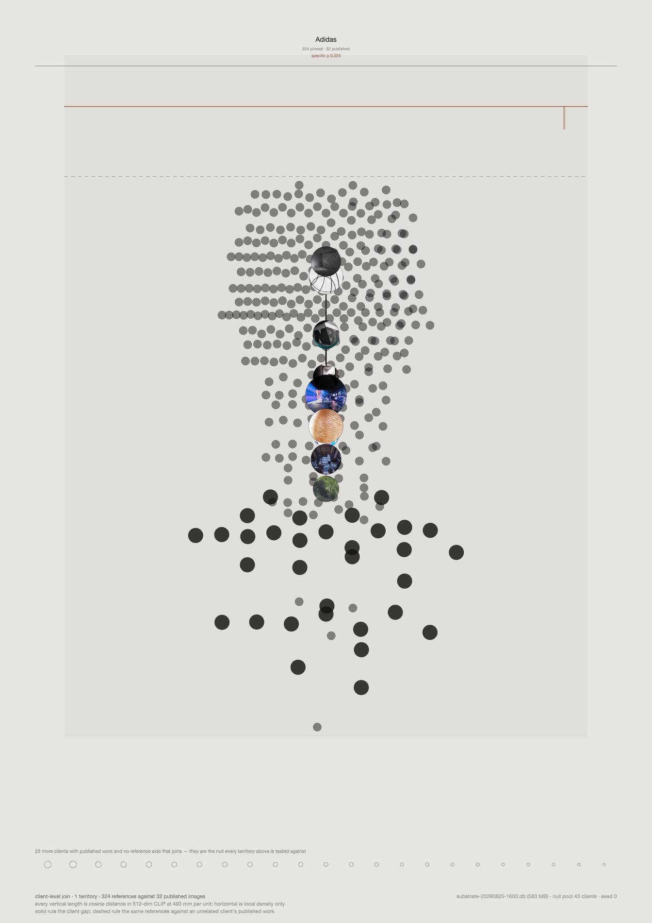
On the composite sheet, one territory is a few centimetres wide and the force paths inside it are hairlines. Here the same territory has a page, and the scale does not change: 556 mm per unit of cosine distance on both sheets, because both are 420 mm tall. So every length here can be laid against the composite with a ruler, which is the one thing a zoom usually destroys.
Adidas is the strongest case in the set and the sheet is drawn solid rather than as a ghost: 0% of its 306 references sit closer to another client's published work than to its own, against 93% at the other end of the table. Its four force paths carry 8, 24, 30 and 44 references and none of them is coloured, meaning no part of this relationship is worse explained by its own research than by an unrelated studio's output.
Vertical position is a real 512-dimension cosine distance at the stated millimetre scale. Horizontal position is local density and nothing else — the horizontal separation of two marks measures nothing at all. There is no t-SNE on this sheet and no length you can put a ruler to that is not a real number.
The solid rule is the client-level gap, 0.038 — the whole-relationship claim. The dashed rule is where the same 306 references sit against an unrelated client's published work, 0.108. The distance between those two lines is the entire evidential content of the territory, and drawing them together is what stops a high pull from being read as a finding on its own.
Twenty-eight clients have published work on field.io and no reference side that joins it. They are not decoration: they are the null pool every territory is tested against, and printing them keeps the test visible next to its result rather than in a footnote.
What would make this wrong. Adidas ranks first of 40 at p = 0.025, which is the permutation floor rather than a small p-value — one client cannot do better than 1/40 on this test, and twelve tests would want 0.0042 to survive Bonferroni. So this is the best-evidenced territory in a collective signal, not a licence to make a claim about Adidas specifically. The isolate also inherits everything the composite says: client-level only, because channel titles match published work on 2 of 166; and no direction, because direction needs a shared two-dimensional basis, which is the projection the sheet exists to avoid.
python3 src/viz/translation_field.py --client Adidas --dpi 200
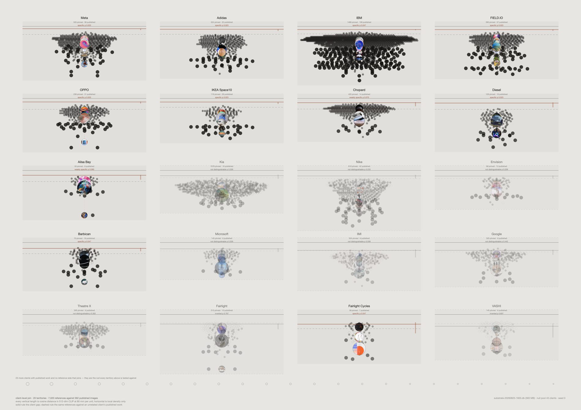
Side by side in one row on the composite sheet, twelve territories read as one gradient and the eye takes the whole thing as evidence. Given a panel each, with the verdict set over the name, the sheet says out loud that half of it is not evidenced: Adidas, OPPO, Diesel and Fairlight Cycles clear p ≤ 0.05; Ailsa Bay and Barbican clear p ≤ 0.10; Meta, Microsoft, Google and Theatre X are indistinguishable from an unrelated client; VASHI and Fairlight sit on the wrong side of their own null, matching other studios' published work more closely than their own, at lift −0.026 and −0.051.
The unmatched share tells the same story more bluntly.
It runs from 0% at Adidas to 93% at Fairlight — the proportion of a client's references that sit closer to at least half of the other 39 clients' published work than to their own. Across all twelve it is 455 of 1,825.
The six territories that do not clear their null are drawn pale rather than dropped. An unevidenced territory is a finding about the join and not an embarrassment to hide, and a sheet that silently kept only its four good cases would be the dishonest version of this one.
Twelve small panels get 167 mm per unit against the composite's 556 — the same geometry drawn 3.3× tighter, because a panel is a third of the page height. Lengths compare panel to panel on this sheet and must not be measured against the main sheet or the isolate. Both sheets print their own scale in the caption for exactly this reason.
Everything the composite has, at panel size: reference cloud, force paths, output cloud, the solid client gap and the dashed unrelated-client baseline. The published cloud stays visibly tighter than the reference cloud in 11 of 12, up to 2.94×. The work is a narrowing of the material, not a move away from it.
What would make this wrong. Small panels flatter a weak signal: at 167 mm per unit a 0.03 lift and a 0.10 lift look more alike than they are, which is why the verdict is printed as text over every panel rather than left to the drawing. The joins are thin under the two-image threshold — six clients rest on 6 to 9 published images — and only 25 of 66 client pairs have 95% intervals that separate, so the left-to-right order of the panels is not a ranking anyone should quote. Cutting every client to six output images shifts the levels by up to 0.036 and leaves the order at Spearman +0.91: the ranking survives, the absolute values do not.
python3 src/viz/translation_field.py --small-multiples --dpi 200
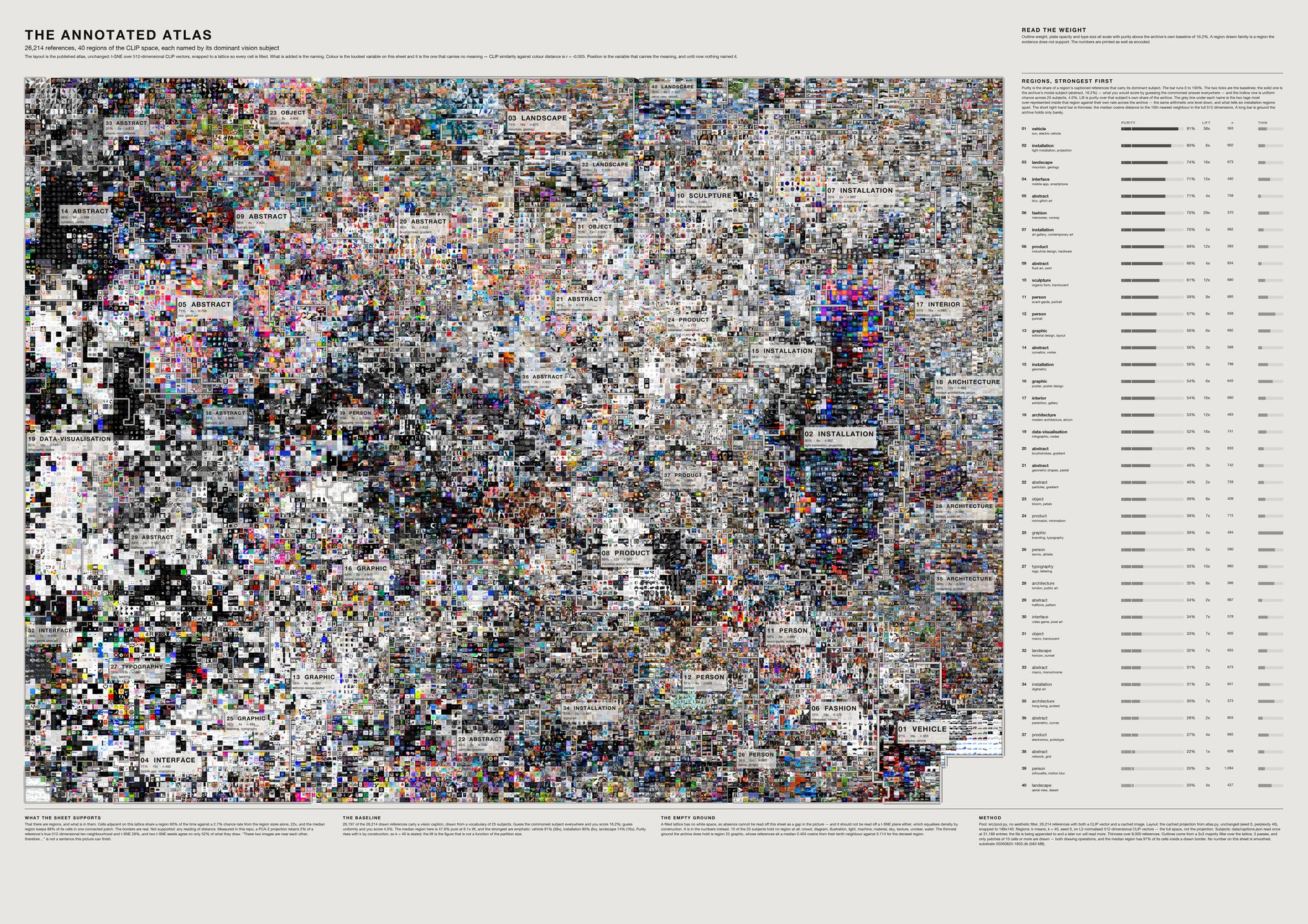
The atlas was a map without a legend, and that is why it read as a colour field. Colour is its loudest variable and the one carrying no meaning: across the archive, CLIP similarity against colour distance is r = −0.005, and CLIP neighbours are only 13.6% closer in colour than chance.
Colour and meaning are near-independent here. Position is what carries the meaning. Cut the CLIP space into 40 regions and each holds a dominant subject at a median purity of 46% against a 12.6% baseline and a 3.7% uniform chance across 27 subjects — a median lift of 7×, reaching 28× for vehicles and 27× for fashion.
Two images in adjacent lattice cells share a region 58.4% of the time, against 2.7% by chance — 22×. Without that the outlines would be decoration over a projection. With it, a region is a real neighbourhood and the border is where it stops.
Six regions share the subject installation and would have been interchangeable. Naming each by its two most over-represented tags separates them: public art, suspended · performance, projection · art gallery, contemporary art · corridor, light art · structure, grid · digital art, exhibition.
t-SNE equalises density by construction, so a white patch on it is a property of the projection and not a gap in the archive. Instead each region carries a thinness bar — median cosine distance to the tenth nearest neighbour in the full 512 dimensions — and nine of 27 subjects hold no territory at all: diagram, illustration, infrastructure, light, material, nature, sky, water, unclear.
What this sheet can and cannot support. PCA-2 retains 2% of a reference's true ten-neighbourhood, t-SNE 28%, and two t-SNE seeds agree on only 52% of what they draw. So it supports "there are regions and here is what they contain". It does not support "these two images sit near each other, therefore…". Purity is drawn three ways and printed as a number so a region at chance draws nothing; smoothing and the patch threshold are drawing operations and cannot move a figure. Captions grew from 26,296 to 27,761 during the render, so a re-run prints slightly different numbers — every figure is computed live and stamped on the sheet.
python3 src/viz/atlas_regions.py --dpi 300
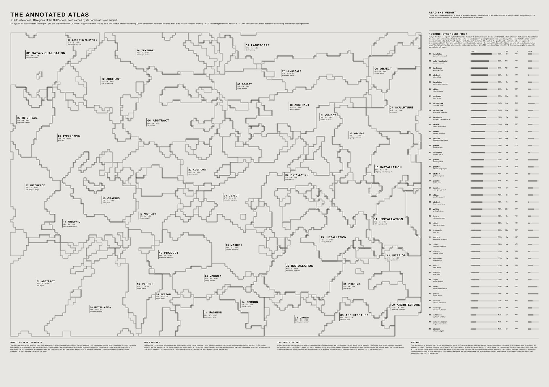
Identical geometry and identical numbers to the sheet above. It exists because at a small size the mosaic wins and the labels stop being readable.
python3 src/viz/atlas_regions.py --no-images --dpi 300
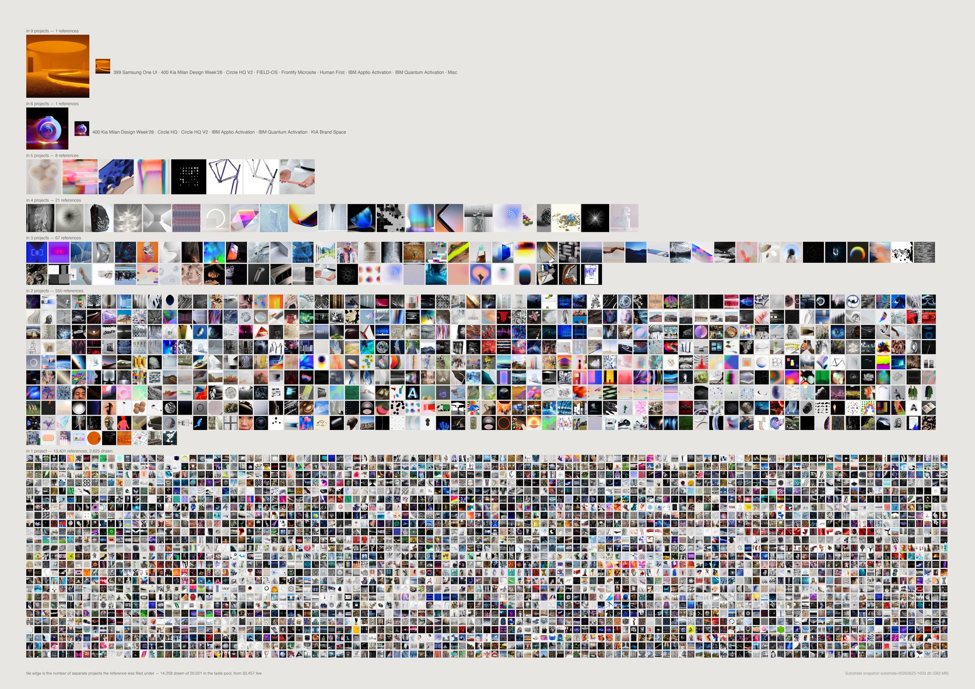
Of 1,636 references in more than one channel, 876 never reach a second project. Being filed under Form and Graphic is tagging, not reuse. Counted across actual jobs, 760 references travelled from one piece of work to another — 4.5% of the 16,786 that reached any project — and the ceiling is five projects, not ten.
Two ways this inflates, both corrected. The raw channel count mixes projects with taxonomy shelves: the most-reused object, a pin called KAV—K, is in 10 channels but 4 jobs and 6 shelves. And sibling channels double-count — 265 Theatre X and 265 Theatre X — Act 1 are siblings, not parent and child, so one pin read as a five-project object when the work was two. Jobs are keyed on number plus first word, because the number alone merges 238 Microsoft x SAP with 238-2 City + Guilds. The second-placed raw object, a pin called network at 9 channels, is in one project.
And the honest limit: channel membership is a proxy for deck membership. Substrate holds no record of the slide itself, so every count here means "somebody put this in that project's research", not "this survived to a slide".
python3 src/viz/reuse.py --dpi 300
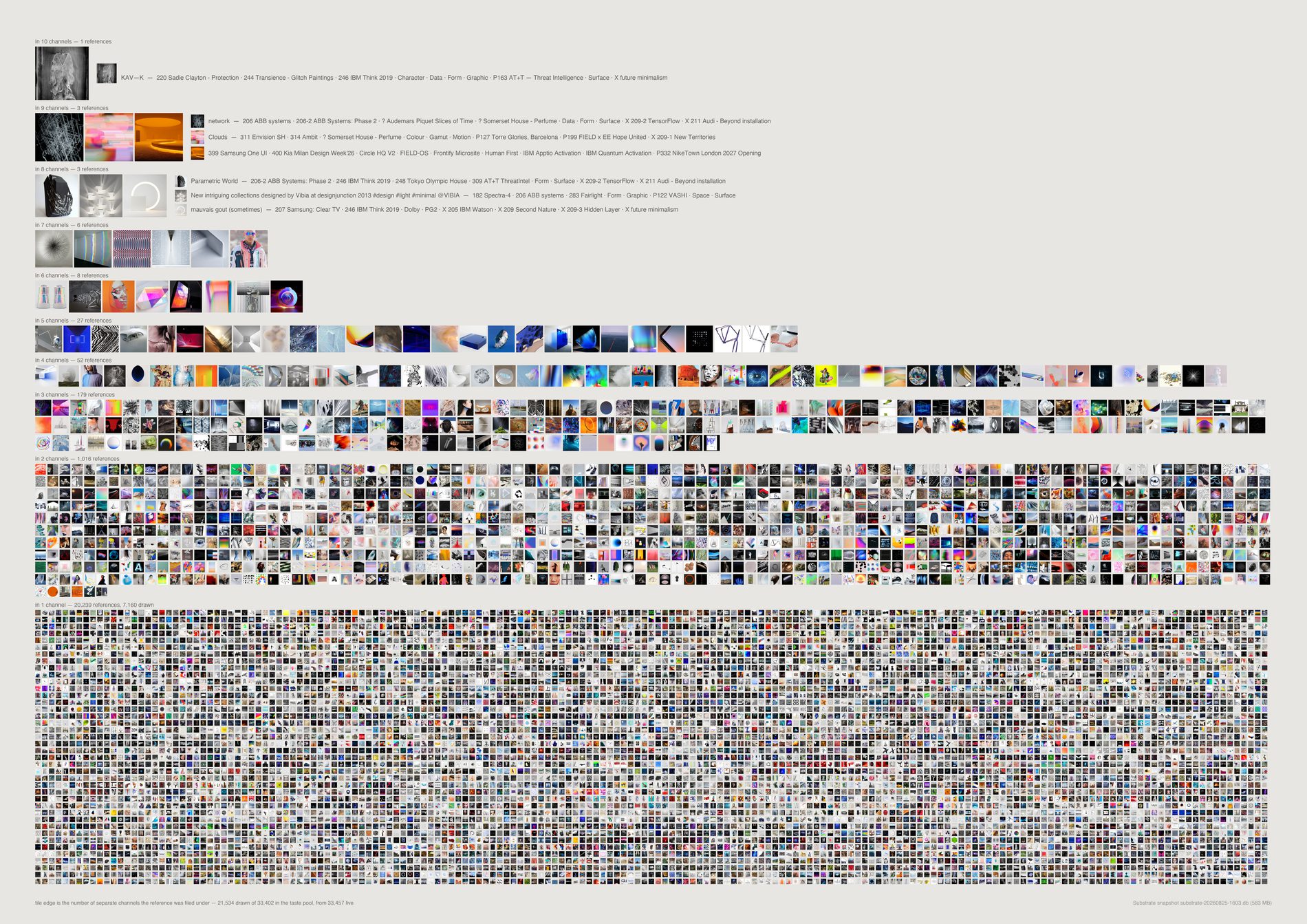
The top seven rows are 24 references out of thirty thousand, and naming their channels is what shows the count to be soft. KAV—K sits in ten: four of them jobs, six of them shelves called Character, Data, Form, Graphic, Surface and X future minimalism. network, at nine, is in one job. 908 references are in exactly two channels and 18,121 in one, so the distribution is not a long tail with a fat head. It is a floor with a few things standing on it.
Why keep an uncorrected sheet on the page. The corrected version folds shelves out and siblings together, and it is the one to quote. This one is the reason to trust that correction: the six shelf names are printed beside the pin, so the inflation is visible rather than asserted. A sheet that only showed the fixed number would be asking to be believed.
python3 src/viz/reuse.py --count channels --out reuse-channels --dpi 300
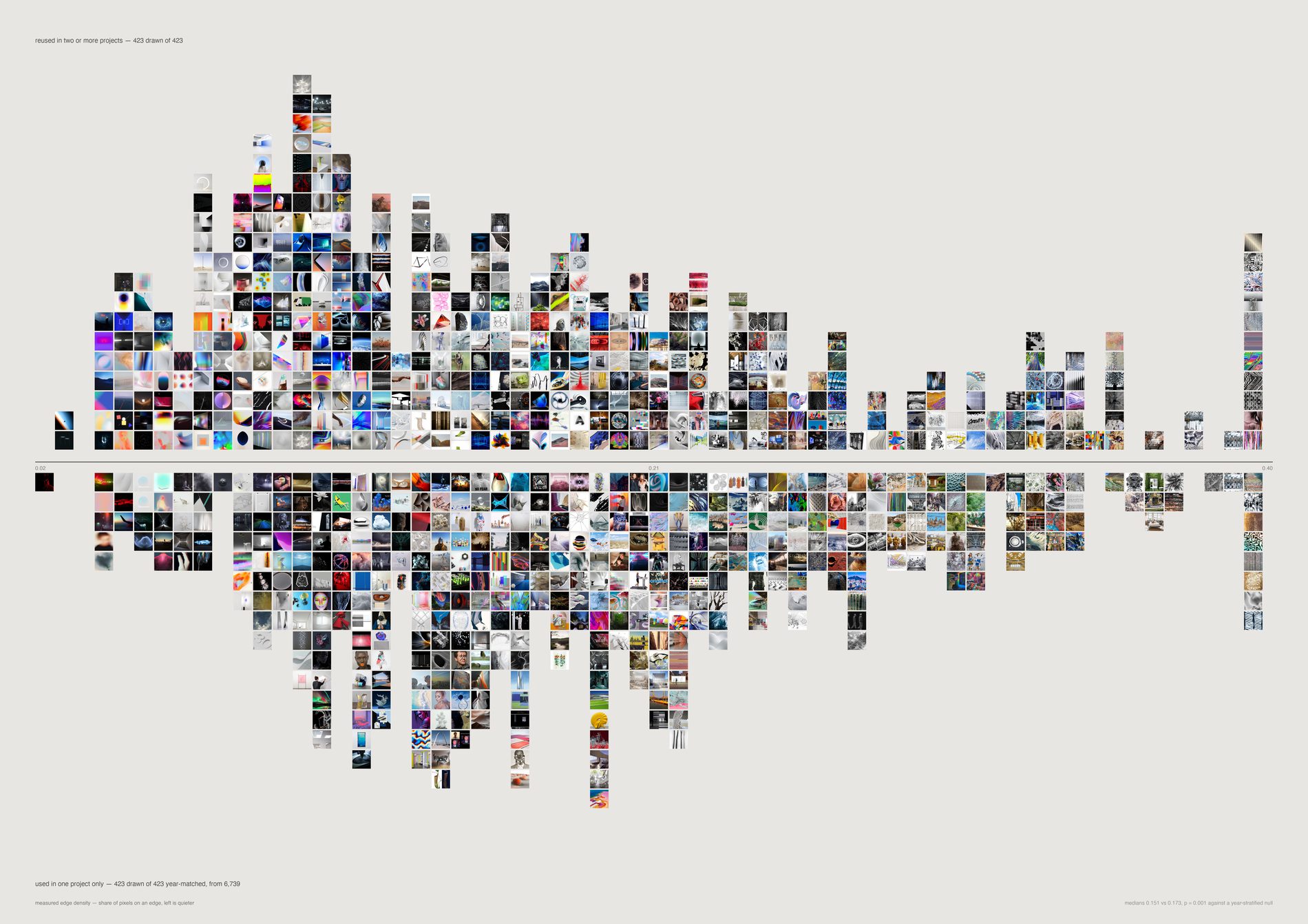
Naively the reused references are quieter, calmer and older — and almost all of that is age. A 2014 pin has had twelve years of decks to appear in, and its reuse rate is 15.4% against 0.9% for 2022 material.
Holding year constant and shuffling 4,000 times, two readings survive: edge density 0.151 against 0.173, p = 0.003, and entropy 6.74 against 6.86, p = 0.023. Saturation, brightness and hue spread do not (p = 0.23, 0.56, 0.32). The studio does not return to calmer colour. It returns to calmer surface.
What would make this wrong. Both survivors held across the re-caption onto a different vision model, which moved the evidence pool underneath them — that is the strongest thing that can be said for them here. But two survivors out of six readings is a narrow result, and it is a statement about Pinterest material only.
python3 src/viz/reuse.py --figure character --out reuse-character --dpi 300
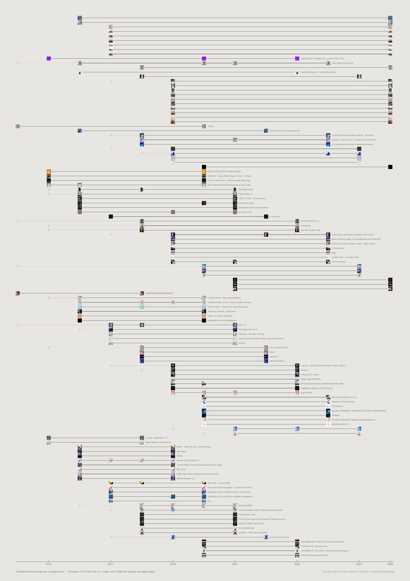
484 references were pulled into work in more than one year. Only 115 span four or more. The longest life belongs to a pin of Nicolas Bernier, found in August 2016, used in Dolby that year and in 400 Kia Milan Design Week’26 a decade later.
A reference used three times in one year is a mood; one reached for across a decade is a conviction.
Dating this needed three attempts and the first two were contaminated. reference_channels.first_observed_at is on all 38,020 rows and is the bulk-import date, not when a reference joined a channel — only 273 references carry more than one value. Channel creation date fails too: 46 of the project channels were created on 25 August, during the Figma ingestion, so anything touching them would read as 2026 work. So would anything filed directly into the Projects and Pitches roots, which carry the import date. The sheet uses a ladder — trustworthy channel date, then project number (year = 0.048n + 2006.9, median residual 0.20 years), then Figma median, then dropped — and prints which rung each job used. The number deliberately outranks the Figma date, because 113 Spring’s frames all carry 2026 from an old file being re-opened, which would have manufactured a ten-year life that never happened.
python3 src/viz/reuse_life.py --page a2 --dpi 300
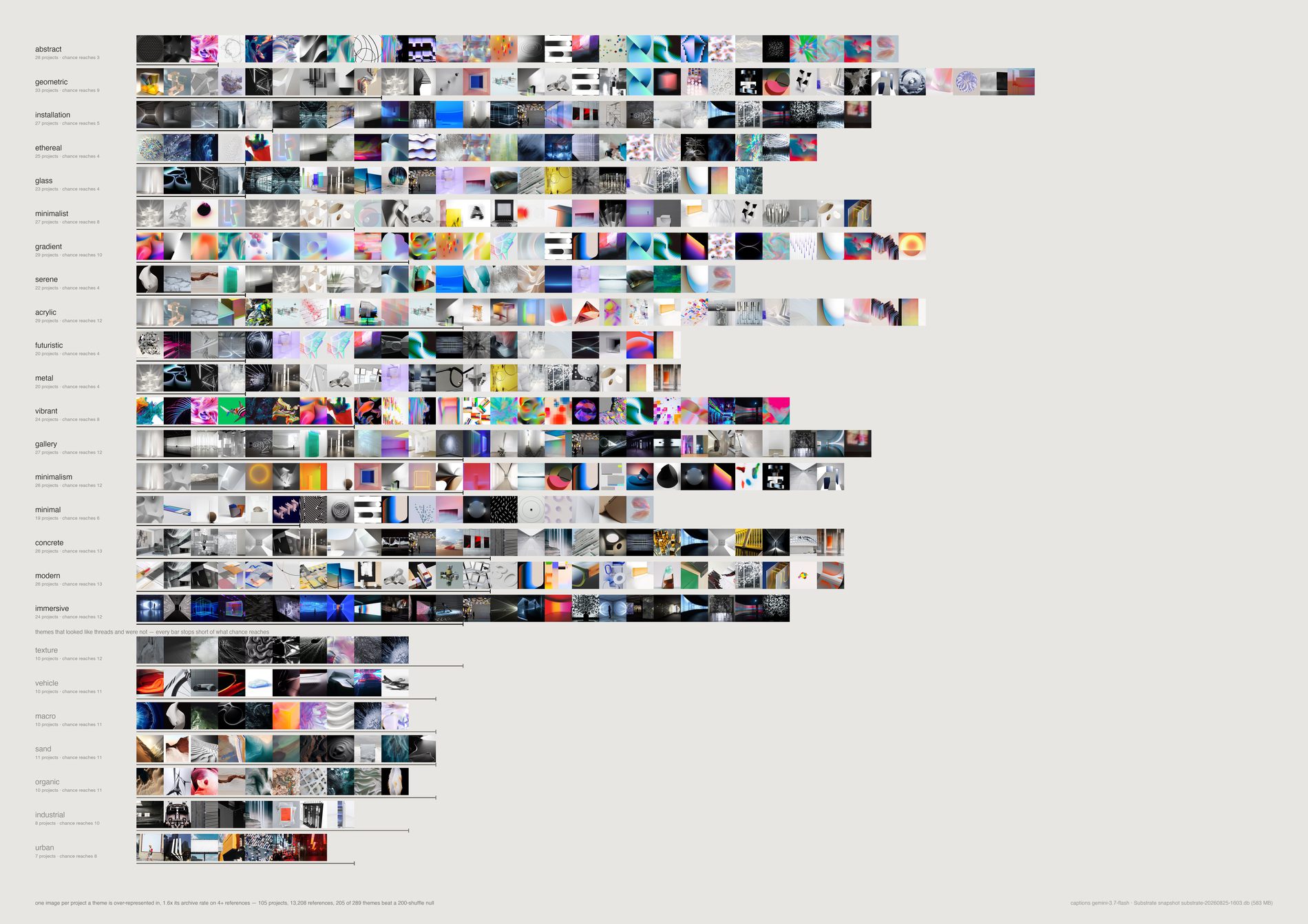
Across 97 projects, abstract is over-represented in 26 where chance reaches 4, installation in 25 against 5, geometric in 29 against 10. The lower band is the more useful half. texture, vehicle, organic, warm, industrial, botanical and urban are everywhere in the work and nowhere more than chance predicts.
They are what the archive is made of, not what the studio keeps reaching for.
Why presence beats frequency. A tag appearing 5,000 times in one project is that project, not a thread. This counts how many separate jobs lean into a theme harder than the archive does, and draws the chance rate beside every bar — so a theme that looks common and isn't distinctive is visibly not a thread rather than quietly omitted.
python3 src/viz/threads.py --dpi 300
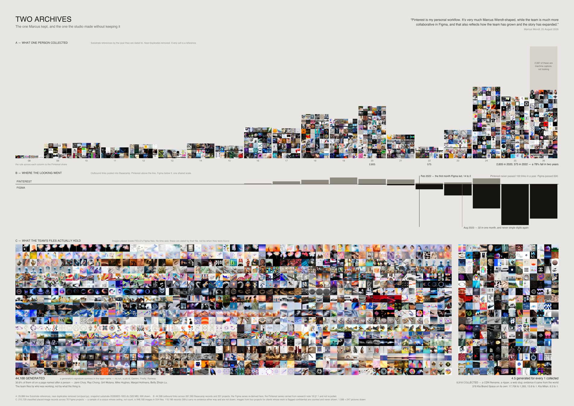
Substrate holds 22,069 live references, and most came off Pinterest — which was Marcus's own habit rather than the studio's. The archive peaks at 2,605 references dated 2020 and falls to 571 by 2022, a 78% drop across exactly the window when Figma overtook Pinterest in Basecamp: February 2022 is the first month Figma led, and by August 2023 it was the default.
The team never stopped collecting. It collected inside a tool that keeps no index, filed under whoever happened to be working — 27.9% of the images in FIELD's Figma files sit on a page named after a person. And most of what is in there now was not collected at all: for every image carrying a trace of having come from the world there are six carrying a generator's signature, and in 378 Kia Brand Space it is closer to fourteen.
References recovered from Figma are dated by when their file first appeared in Basecamp, not by when the image was found. Plotted on a timeline they would manufacture a dramatic recent surge that is an artefact of the import. So the top register uses each reference's own date and nothing file-dated appears on a time axis anywhere on this sheet.
Three figures from the earlier survey are restated here from a larger sample: person-named pages 34.3% → 27.9%, generated share 18.2% → 26.4%, collected share 9.45% → 4.4%. The survey counted 9,017 distinct layer names; this counts every classified placed-image record. Bigger sample, different unit — and the ratio it implies is worse, not better.
What would make this wrong. The 2026 column is drawn with a flat block where its 2,087 machine-captured references sit, so its height is honest and its content is visibly not looking — the recent rebound is a capture agent, not behaviour. The Basecamp Pinterest series is carried from the migration survey rather than re-pulled; the Figma series was re-derived row by row. The Figma corpus was still growing while this was drawn (52 → 57 projects during the run), so every ratio is computed at draw time and printed in the caption. Four Figma projects belong to clients whose published work is flagged confidential — their images are counted and never drawn. And the correlation is not proof of the cause: Google A Space for Being and On Running NYC have no references and no Figma links, because they predate Figma entirely.
python3 src/viz/two_archives.py --dpi 300
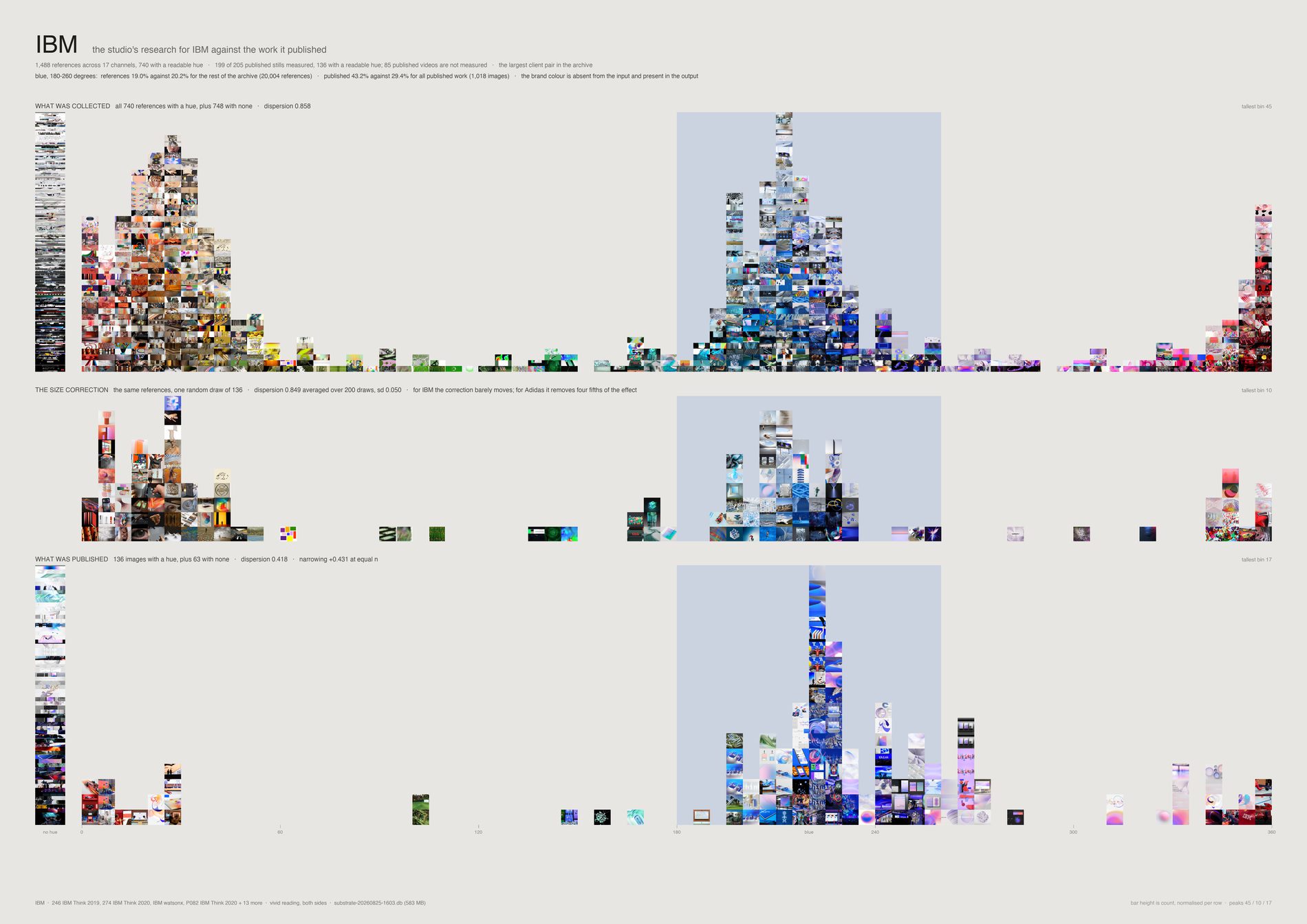
vivid measurement on both sidesThe brand colour lives in the output, not the input. IBM's references are 18.2% blue against 20.5% for the rest of the archive — very slightly less blue.
Its published work is 43.2% against 29.4% for all published work. Hue dispersion falls from 0.874 to 0.418, a narrowing of +0.456. The studio does not collect IBM blue in order to make IBM work; it collects something else, and the blue arrives in the making.
What would make this wrong. Achromatic images are counted in their own column rather than dropped — IBM has 461 of them against 379 carrying a hue — because a sheet about colour that silently discards the greys is measuring its own filter. 85 published IBM videos are unmeasured. And this is one colour system throughout, the vivid reading; the repo measures colour three different ways and they must never be mixed on one sheet.
python3 src/viz/convergence.py --sheet ibm --dpi 300
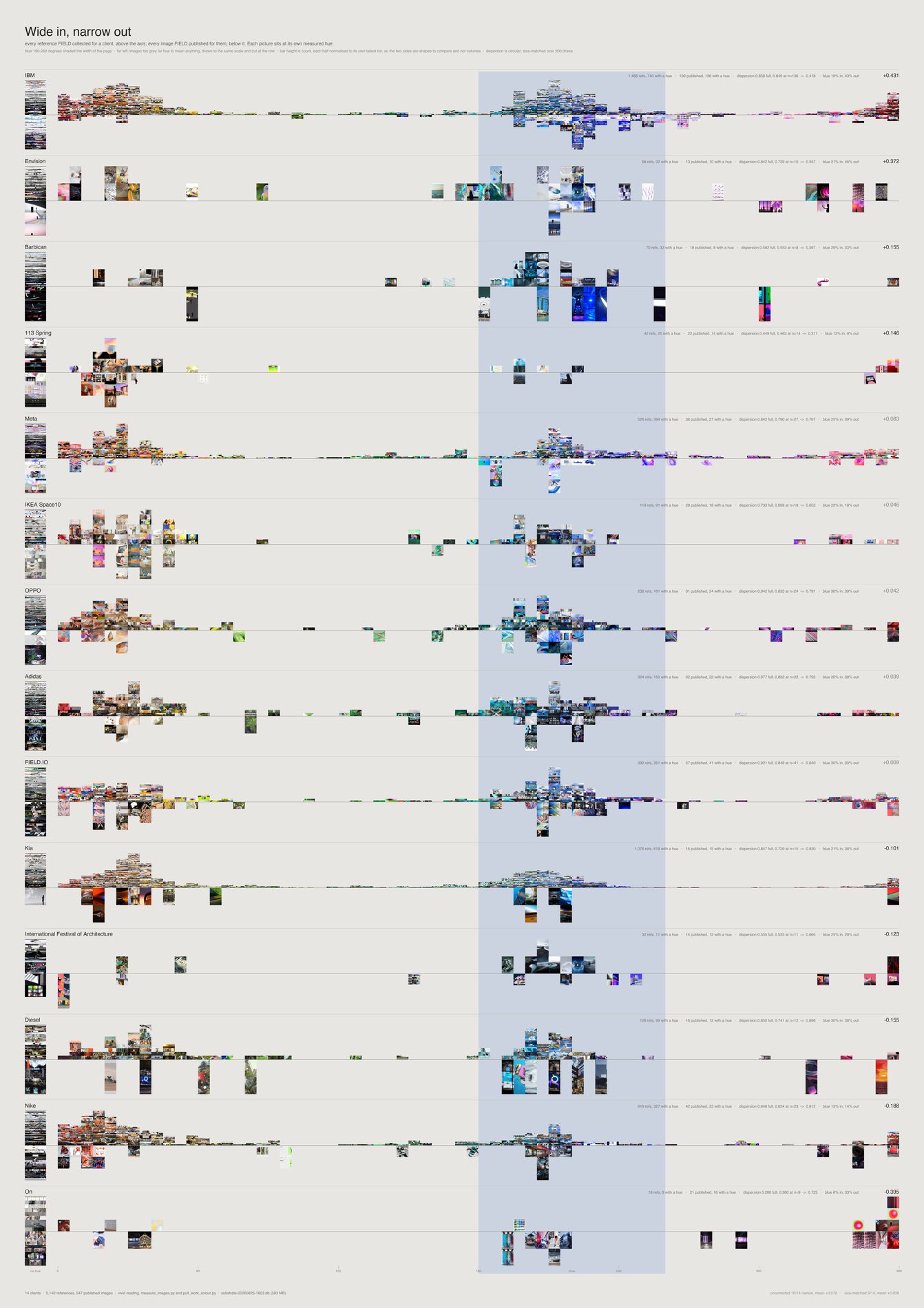
8 of 12 clients narrow — and 8 of 12 still narrow after the correction, so the count is not the story. The magnitude is. Mean narrowing falls from +0.093 to +0.040 once the reference side is subsampled to the published side's size.
Adidas keeps a fifth of its apparent narrowing, OPPO a quarter. Only IBM (+0.456), Envision (+0.381) and Barbican (+0.155) are large. On (−0.314), Diesel (−0.144) and Kia (−0.108) run the other way and expand.
What would make this wrong. Nike looks like the strongest counter-example and cannot be used as one: its channel holds 36 references, 18 after the pool, and 5 carrying any chroma at all — a dispersion over five colours is not a measurement. It falls below the floor and is excluded on the same rule as everyone else. The claim this sheet supports is not "FIELD converges on brand colour" but "where a client has a strong colour identity the output converges on it while the research does not, and the effect is client-specific".
python3 src/viz/convergence.py --sheet clients --dpi 300
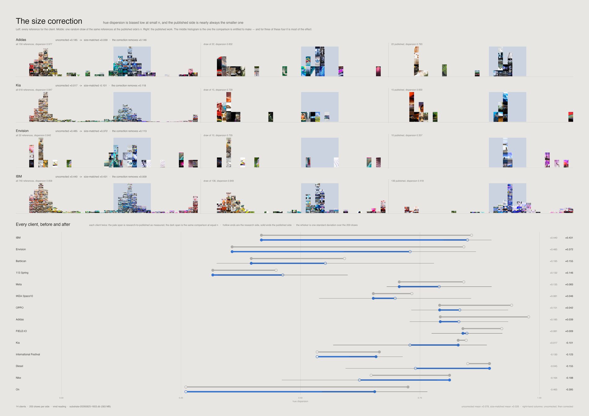
Dispersion estimated from a small sample runs low whatever the underlying distribution, and the published side of every client is smaller than its reference side. Subsampling the references to the published n, 200 draws each, removes that bias. More than half the studio-wide effect disappears with it. The correction is drawn rather than described, because the uncorrected sheet is the one a reader would otherwise believe.
Why this is on the page at all. This project has published two findings that turned out to be artefacts of how they were measured — a hole in the archive that was the smoothest point on its sheet, and a null whose test could not have detected the thing it declared absent. Drawing the correction is cheaper than another retraction.
python3 src/viz/convergence.py --sheet correction --dpi 300
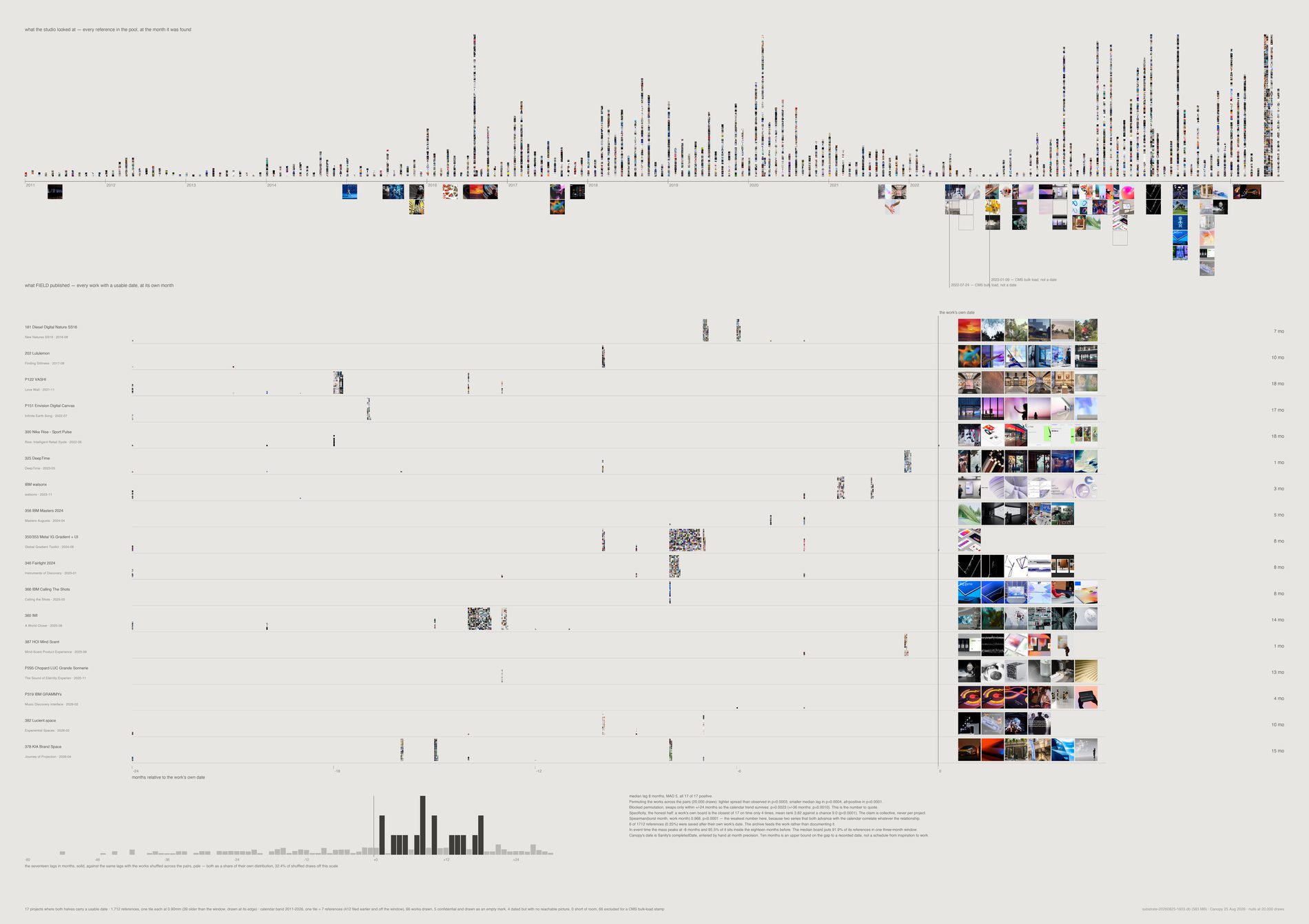
17 of 17 lags are positive, median 10 months, range 1–18. Only 2 of 877 references (0.23%) were saved after their own project's work was dated — so the archive feeds the work rather than documenting it, and that is a measured number rather than a reassurance.
A board is a sprint: the median project puts 93.8% of its references inside a single three-month window, and in event time the mass peaks at −10 months with 95.2% inside the eighteen months before.
Permuting works across pairs gives p = 0.0003, but that destroys the calendar trend and two series both advancing with time will correlate whatever their relationship. The honest test is the blocked permutation, swapping only between works dated within ±24 months, which preserves the trend: p = 0.0149. That is the number to quote.
Asked which of the 17 boards sits closest in time to a given work, the work's own board wins only 4 of 17 — mean rank 3.94 against a chance 9.0. Real, and far weaker than the collective claim. Several jobs run at once and their bursts overlap, so timing alone cannot tell you which board fed which brief. The sheet is drawn as a distribution, not as 17 verdicts.
What would make this wrong. Canopy's date is Sanity's completedDate, hand-entered at month precision — 71 of 75 usable values carry no time, 16 calendar days hold two or more works — and it is ambiguous between finished and put on the website. So "ten months from inspiration to work" is not supported; only that the looking is over roughly ten months before the recorded date. Everything is rounded to months for that reason. And 66 of 141 works cannot be timed at all, because two bulk-import days carry 66 of them between them.
python3 src/viz/incubation.py --dpi 300
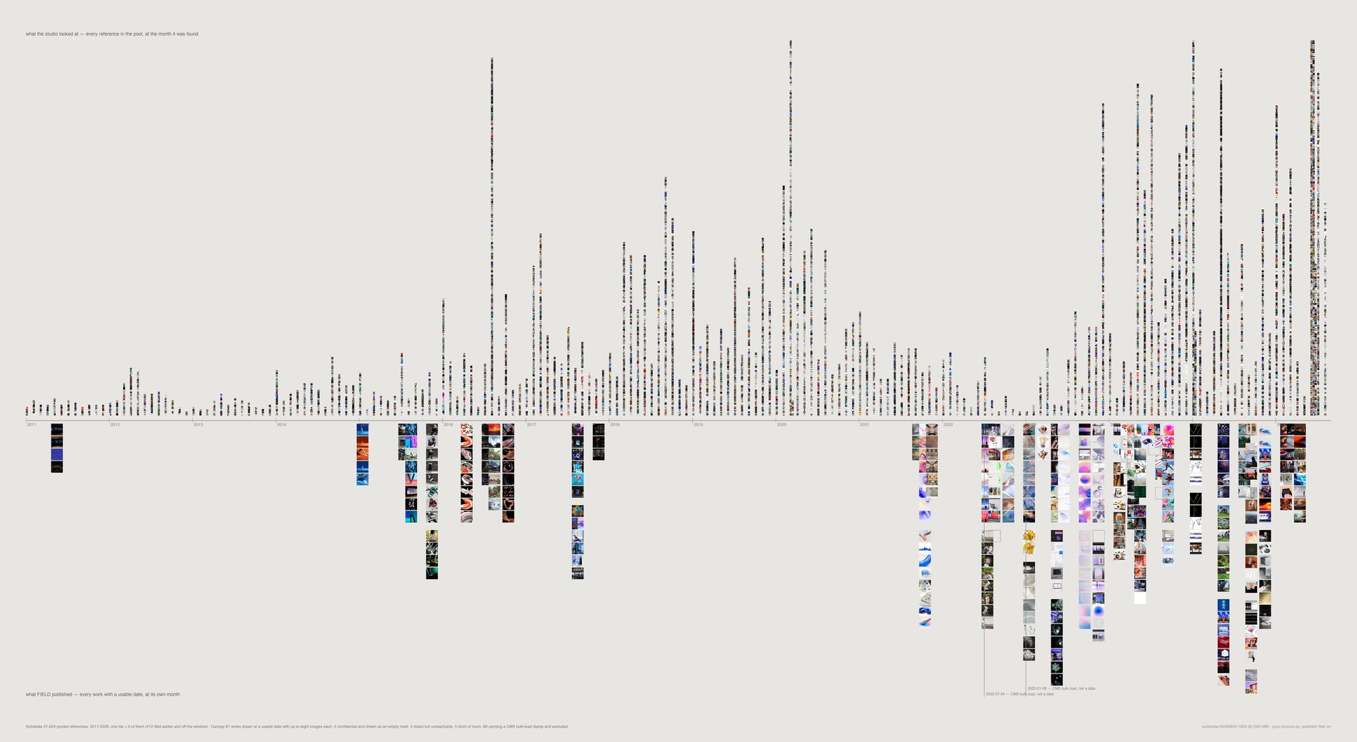
The intake collapse is visible here without being argued: the archive falls from 3,168 references dated 2020 to 688 dated 2022, across exactly the window in which the studio moved from Pinterest to Figma. February 2022 is the measured crossover, and the 2026 rebound is machinery — a capture agent and a one-off import — rather than behaviour.
Confidential work is named but never shown. Five flagged works have usable dates and appear as empty outline marks, counted separately from the four genuine cache failures so the caption does not conflate a policy with a broken image.
python3 src/viz/incubation.py --sheet calendar --out incubation-calendar --dpi 300